
Loading article…
|
確率密度関数 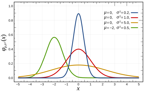 赤い曲線は標準正規分布です。 | |||
|
累積分布関数 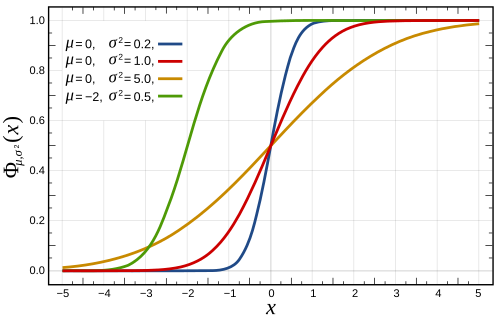 | |||
| 表記 | |||
|---|---|---|---|
| パラメータ |
=平均(位置) =分散( 二乗スケール) | ||
| サポート | |||
| ドイツ連邦共和国 | |||
| クォンタイル | |||
| 平均 | |||
| 中央値 | |||
| モード | |||
| 分散 | |||
| 狂った | |||
| 歪度 | |||
| 過剰尖度 | |||
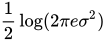
| エントロピ | |||
| MGF の | |||
| CF | |||
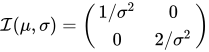
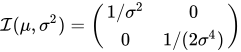
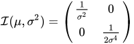
| フィッシャー情報 |
| ||
| カルバック・ライブラー距離 | |||
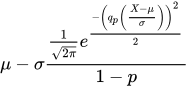
| 予想される不足額 | [1] | ||


![{\displaystyle \Phi \left({\frac {x-\mu }{\sigma }}\right)={\frac {1}{2}}\left[1+\operatorname {erf} \left({\frac {x-\mu }{\sigma {\sqrt {2}}}}\right)\right]}](https://wikimedia.org/api/rest_v1/media/math/render/svg/c0fed43e25966344745178c406f04b15d0fa3783)






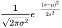
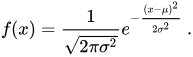
確率論と統計学において、正規分布またはガウス分布は、実数値のランダム変数に対する連続確率分布の一種です。その確率密度関数の一般的な形式はです。 パラメータ は分布の平均または期待値(および中央値と最頻値)であり、パラメータは分散です。分布の標準偏差は(シグマ) です。ガウス分布のランダム変数は正規分布していると言われ、正規偏差と呼ばれます。


正規分布は統計学において重要であり、分布が不明な実数値のランダム変数を表すために自然科学や社会科学でよく使用されます。 [2] [3]正規分布の重要性は、中心極限定理に一部起因しています。中心極限定理は、ある条件下では、有限の平均と分散を持つランダム変数の多数のサンプル(観測値)の平均は、それ自体がランダム変数であり、その分布はサンプル数が増えるにつれて正規分布に収束することを述べています。したがって、測定誤差などの多くの独立したプロセスの合計であると予想される物理量は、ほぼ正規分布になることがよくあります。[4]
さらに、ガウス分布には、分析研究に役立ついくつかのユニークな特性があります。たとえば、独立した正規偏差の固定された集合の任意の線形結合は、正規偏差です。不確実性の伝播や最小二乗法[5]パラメータフィッティングなどの多くの結果と方法は、関連する変数が正規分布している場合、明示的な形式で分析的に導くことができます。
正規分布は非公式にはベル曲線と呼ばれることもあります。[6]しかし、ベル曲線の形をした分布は他にもたくさんあります(コーシー分布、スチューデントのt分布、ロジスティック分布など)。その他の名前については命名を参照してください。
単変量確率分布は、多変量正規分布のベクトルと行列正規分布の行列に対して一般化されます。
定義
標準正規分布
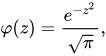
正規分布の最も単純なケースは、標準正規分布または単位正規分布として知られています。これは、およびの場合の特殊なケースであり、次の確率密度関数(または密度)によって記述されます。 変数の平均は 0、分散と標準偏差は 1 です。密度はでピークを持ち、とで変曲点を持ちます。


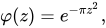
上記の密度は標準正規分布として最もよく知られていますが、他のバージョンの正規分布を説明するためにこの用語を使用している著者もいます。たとえば、 カール・フリードリヒ・ガウスはかつて標準正規分布を の分散を持つと定義し、スティーブン・スティグラー[7]はかつて標準正規分布を の単純な関数形式で分散を持つと定義しました。


一般正規分布
すべての正規分布は標準正規分布のバージョンであり、その定義域は係数(標準偏差)によって引き伸ばされ、次に係数 (平均値) によって変換されます。

確率密度は、積分が 1 のままになるようにスケーリングする必要があります。

が標準正規偏差である場合、 は期待値と標準偏差の正規分布を持ちます。これは、標準正規分布をの係数で拡大/縮小し、 だけシフトして、と呼ばれる別の正規分布を生成できるということと同じです。逆に、 がパラメータおよびの正規偏差である場合、この分布は、式を使用して再拡大縮小およびシフトし、標準正規分布に変換できます。この変量は の標準化された形式とも呼ばれます。



表記
標準ガウス分布(平均ゼロ、分散1の標準正規分布)の確率密度は、ギリシャ文字の(ファイ)で表されることが多い。[8]ギリシャ文字ファイの代替形である もよく使われる。


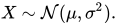
正規分布はしばしばまたはと呼ばれる。[9]したがって、ランダム変数が平均と標準偏差で正規分布している場合、次のように書くことができる。


代替パラメータ化
標準偏差や分散の代わりに、分布の幅を定義するパラメータとして精度 を使用することを主張する著者もいる。精度は通常、分散の逆数として定義される。[ 10]分布の式は次のようになる。


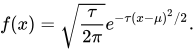
この選択は、 がゼロに非常に近い場合の数値計算で利点があり、多変量正規分布を持つ変数のベイズ推定などのいくつかのコンテキストで式を簡素化すると主張されています。
あるいは、標準偏差の逆数を精度として定義すると、正規分布の式は次のようになる。


スティグラーによれば、この定式化は、式がはるかに単純で覚えやすく、分布の 分位数の近似式が単純であるため有利です。
正規分布は、自然パラメータおよび、自然統計量xおよびx 2を持つ指数族を形成します。正規分布の双対期待パラメータは、η 1 = μおよびη 2 = μ 2 + σ 2です。


累積分布関数
標準正規分布の累積分布関数( CDF)は、通常ギリシャ文字の大文字(ファイ)で表され、積分である。


エラー関数
関連する誤差関数は 、平均 0 および分散 1/2 の正規分布に従うランダム変数が範囲 に入る確率を与えます。つまり、

![{\textstyle [-x,x]}](https://wikimedia.org/api/rest_v1/media/math/render/svg/4939f2eb7c55ff4e7d13331fc0599a5f2452b479)

これらの積分は初等関数では表現できず、特殊関数と呼ばれることが多い。しかし、多くの数値近似が知られている。詳細については以下を参照。
2つの機能は密接に関連しており、
![{\displaystyle \Phi (x)={\frac {1}{2}}\left[1+\operatorname {erf} \left({\frac {x}{\sqrt {2}}}\right)\right]\,.}](https://wikimedia.org/api/rest_v1/media/math/render/svg/4dec6de19ebeaa734086622f167d87ac41e7b50d)
密度、平均、分散を持つ一般的な正規分布の場合、累積分布関数は

![{\displaystyle F(x)=\Phi \left({\frac {x-\mu }{\sigma }}\right)={\frac {1}{2}}\left[1+\operatorname {erf} \left({\frac {x-\mu }{\sigma {\sqrt {2}}}}\right)\right]\,.}](https://wikimedia.org/api/rest_v1/media/math/render/svg/f48cf2d3b65754e434e6a6c5a90908dd83d44f12)
標準正規累積分布関数の補関数は、特に工学の教科書ではQ関数と呼ばれることが多い。 [11] [12]これは、標準正規乱数変数の値がを超える確率を与える。関数の他の定義(すべて の単純な変換)も時々使用される。[13]


標準正規累積分布関数のグラフは、点(0,1/2)を中心に2回回転対称性を持ちます。つまり、 です。その不定積分は次のように表すことができます。


標準正規分布の累積分布関数は、部分積分によって級数に展開できます。
![{\displaystyle \Phi (x)={\frac {1}{2}}+{\frac {1}{\sqrt {2\pi }}}\cdot e^{-x^{2}/2}\left[x+{\frac {x^{3}}{3}}+{\frac {x^{5}}{3\cdot 5}}+\cdots +{\frac {x^{2n+1}}{(2n+1)!!}}+\cdots \right]\,.}](https://wikimedia.org/api/rest_v1/media/math/render/svg/ad8275ec6180f68c2dae03c9e70716b75ff4f3aa)
ここで は二重階乗を表します。

大きなxに対する累積分布関数の漸近展開も部分積分を使って導くことができる。詳しくは誤差関数#漸近展開を参照のこと。[14]
標準正規分布の累積分布関数の近似値は、テイラー級数近似を使用して簡単に求めることができます。

テイラー級数展開による再帰計算
導関数族の再帰的性質は、分布の既知の値の任意の点についての再帰的要素を使用して、急速に収束するテイラー級数展開を簡単に構築するために使用できます。


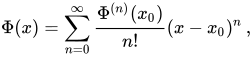
どこ:

逆関数にテイラー級数とニュートン法を使用する
上記のテイラー級数展開の応用として、ニュートン法を使用して計算を逆にすることができます。つまり、累積分布関数の値が分かっているが、を取得するために必要な x が分からない場合は、ニュートン法を使用して x を見つけ、上記のテイラー級数展開を使用して計算回数を最小限に抑えることができます。ニュートン法は、 の 1 次導関数 (正規標準分布の積分) が正規標準分布であり、ニュートン法のソリューションですぐに使用できるため、この問題を解決するのに最適です。

解決するには、目的の に対する既知の近似解 を選択してください。 は分布表の値、または任意の計算方法を使用して を計算した後のインテリジェント推定値である可能性があります。 のこの値と上記のテイラー級数展開を使用して、計算を最小限に抑えます。

計算されたと目的の の差 ( と呼ぶ)が、10 −5、10 −15などの許容可能な小さい誤差より小さくなるまで、次のプロセスを繰り返します。


どこ
- は、テイラー級数解からであり、


繰り返し計算が、選択された許容可能な小さい値以下の誤差に収束すると、x は目的の値のa を取得するために必要な値になります。
標準偏差とカバレッジ
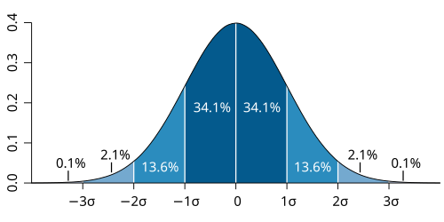
正規分布から抽出された値の約68%は平均値から1標準偏差σ以内にあり、約95%は2標準偏差以内にあり、約99.7%は3標準偏差以内にあります。[6]この事実は、68-95-99.7(経験的)ルール、または3シグマルールとして知られています。
より正確には、正規分布が から までの範囲にある確率はで与えられます 。 12 桁の有効数字の場合、 の値は次のようになります。




が大きい場合は、近似値 を使用できます。


分位関数
分布の分位関数は、累積分布関数の逆です。標準正規分布の分位関数はプロビット関数と呼ばれ、逆誤差関数で表すことができます。 平均と分散 の正規ランダム変数の場合、分位関数 は です。標準正規分布の分位は通常 と表されます 。これらの値は、仮説検定、信頼区間の構築、Q-Q プロットで使用されます。正規ランダム変数はの確率で を超え、の確率で区間外になります。特に、分位点は1.96であるため、正規ランダム変数が区間外になるのは 5% のケースのみです。




次の表は、指定された確率で範囲に入る分位数を示しています。これらの値は、正規分布(または漸近正規分布)を持つサンプル平均やその他の統計的推定値の許容区間を決定するのに役立ちます。[15]次の表は、上記の定義とは異なります。


が小さい場合、分位関数は有用な漸近展開を持つ[要出典]

プロパティ
正規分布は、最初の2つ(つまり、平均と分散以外)を超えるキュムラントがゼロになる唯一の分布です。また、指定された平均と分散に対して最大エントロピーを持つ連続分布でもあります。[16] [17] Gearyは、平均と分散が有限であると仮定すると、独立した一連の抽出から計算された平均と分散が互いに独立している唯一の分布は正規分布であることを示しました。[18] [19]
正規分布は楕円分布のサブクラスです。正規分布は平均に関して対称で、実数線全体にわたって非ゼロです。そのため、人の体重や株価など、本質的に正または大きく歪んだ変数には適したモデルではない場合があります。このような変数は、対数正規分布やパレート分布などの他の分布によってより適切に説明される場合があります。
正規分布の値は、平均値から数標準偏差以上離れている場合、実質的にゼロになります (たとえば、3 標準偏差の広がりは、分布全体の 0.27% を除くすべてをカバーします)。したがって、外れ値 (平均値から多くの標準偏差離れた値) がかなりの割合で存在すると予想される場合、このモデルは適切ではない可能性があります。また、正規分布する変数に最適な最小二乗法やその他の統計的推論法は、そのようなデータに適用すると、信頼性が非常に低くなることがよくあります。このような場合は、より裾の重い分布を想定し、適切な堅牢な統計的推論法を適用する必要があります。
ガウス分布は、平均や分散が有限であるかどうかに関係なく、独立した同一分布の和のアトラクターである安定分布のファミリーに属します。極限の場合であるガウス分布を除いて、すべての安定分布は重い裾と無限の分散を持ちます。これは、安定しており、解析的に表現できる確率密度関数を持つ数少ない分布の 1 つであり、他の分布はコーシー分布とレヴィ分布です。
対称性と微分
密度(平均と分散)を持つ正規分布には、次の特性があります。


- これは分布の最頻値、中央値、平均値である点を中心に対称である。 [20]
- これは単峰性であり、1次導関数はに対しては正、に対しては負で、 に対してのみゼロである。
- 曲線と- 軸によって囲まれた領域は 1 です (つまり 1 に等しい)。
- その一次導関数は
- その2次導関数は
- その密度には2つの変曲点(2次導関数がゼロで符号が変わる点)があり、平均値から1標準偏差離れたところ、つまりとにある[ 20]
- その密度は対数凹面である。[20]
- その密度は無限に微分可能であり、実際2次の超滑らかさである。[21]


さらに、標準正規分布の密度(つまり、および)には次の特性もあります。

- その一次導関数は
- その2次導関数は
- より一般的には、そのn次導関数はn次(確率論的)エルミート多項式である。[22]
- 正規分布する変数が既知であり、特定のセット内にある確率は、分数が標準正規分布に従うという事実を使用して計算できます。


瞬間
変数の単純モーメントと絶対モーメントは、それぞれ との期待値です。の期待値が 0 の場合、これらのパラメータは中心モーメントと呼ばれます。それ以外の場合は、これらのパラメータは非中心モーメントと呼ばれます。通常、整数次 のモーメントのみを対象とします。


が正規分布に従う場合、非中心モーメントは存在し、実部が−1より大きい任意のものに対して有限である。任意の非負整数 に対して、単純中心モーメントは次のようになる。[23] ここで は二重階乗、つまり から 1 までのすべての数の積を表し、 と同じ偶奇性を持つ。
![{\displaystyle \operatorname {E} \left[(X-\mu )^{p}\right]={\begin{cases}0&{\text{p{\text{が奇数の場合、}}\\\sigma ^{p}(p-1)!!&{\text{p{\text{が偶数の場合。}}\end{cases}}}](https://wikimedia.org/api/rest_v1/media/math/render/svg/f1d2c92b62ac2bbe07a8e475faac29c8cc5f7755)


中心絶対モーメントはすべての偶数次数では平モーメントと一致するが、奇数次数ではゼロではない。任意の非負整数に対して

最後の式は、任意の非整数に対しても有効である。平均が、平積率と絶対積率を合流型超幾何関数で表すことができる場合、[24]
![{\displaystyle {\begin{aligned}\operatorname {E} \left[|X-\mu |^{p}\right]&=\sigma ^{p}(p-1)!!\cdot {\begin{cases}{\sqrt {\frac {2}{\pi }}}&{\text{if }}p{\text{ is odd}}\\1&{\text{if }}p{\text{ is even}}\end{cases}}\\&=\sigma ^{p}\cdot {\frac {2^{p/2}\Gamma \left({\frac {p+1}{2}}\right)}{\sqrt {\pi }}}.\end{aligned}}}](https://wikimedia.org/api/rest_v1/media/math/render/svg/3b196371c491676efa7ea7770ef56773db7652cd)


![{\displaystyle {\begin{aligned}\operatorname {E} \left[X^{p}\right]&=\sigma ^{p}\cdot (-i{\sqrt {2}})^{p}U\left(-{\frac {p}{2}},{\frac {1}{2}},-{\frac {1}{2}}\left({\frac {\mu }{\sigma }}\right)^{2}\right),\\\operatorname {E} \left[|X|^{p}\right]&=\sigma ^{p}\cdot 2^{p/2}{\frac {\Gamma \left({\frac {1+p}{2}}\right)}{\sqrt {\pi }}}{}_{1}F_{1}\left(-{\frac {p}{2}},{\frac {1}{2}},-{\frac {1}{2}}\left({\frac {\mu }{\sigma }}\right)^{2}\right).\end{aligned}}}](https://wikimedia.org/api/rest_v1/media/math/render/svg/0c17bf881593b86e728bf5dfbdb41a4b86da3875)
これらの式は、 が整数でない場合でも有効です。一般化エルミート多項式も参照してください。
区間内にあるイベントを条件とするの期待値は で与えられます 。 ここで、 と はそれぞれ の密度と累積分布関数です。これは逆ミルズ比として知られています。上記では、逆ミルズ比のように標準正規密度の代わりに の密度が使用されていることに注意してください。そのため、ここではの代わりに が使用されています。
![{\textstyle [a,b]}](https://wikimedia.org/api/rest_v1/media/math/render/svg/2c780cbaafb5b1d4a6912aa65d2b0b1982097108)
![{\displaystyle \operatorname {E} \left[X\mid a<X<b\right]=\mu -\sigma ^{2}{\frac {f(b)-f(a)}{F(b)-F(a)}}\,,}](https://wikimedia.org/api/rest_v1/media/math/render/svg/ad97cc40960e6d1d4e65f51596c9cd0c9accfdc0)


フーリエ変換と特性関数
平均と分散を持つ正規密度のフーリエ変換は[25]

ここで、 は虚数単位です。平均 の場合、最初の因子は 1 であり、フーリエ変換は、定数因子を除けば、平均 0 および分散 の周波数領域上の正規密度です。特に、標準正規分布はフーリエ変換の 固有関数です。

確率論では、実数値ランダム変数の確率分布のフーリエ変換は、その変数の特性関数と密接に関係しており、特性関数は実変数(フーリエ変換の周波数パラメータ)の関数としての の期待値として定義されます。この定義は、複素数値変数 に解析的に拡張できます。[26]両者の関係は次のとおりです。


モーメントとキュムラントを生成する関数
実数ランダム変数のモーメント生成関数は、実パラメータの関数としてのの期待値です。密度、平均、分散を持つ正規分布の場合、モーメント生成関数が存在し、次の式に等しくなります。

任意の について、モーメント生成関数 ( の指数級数として表される) における の係数は、正規分布の期待値 です。
![{\displaystyle M(t)=\operatorname {E} \left[e^{tX}\right]={\hat {f}}(it)=e^{\mu t}e^{\sigma ^{2}t^{2}/2}\,.}](https://wikimedia.org/api/rest_v1/media/math/render/svg/3b5930b107fb4328bc04d077d65ce3d2bf1510de)


![{\displaystyle E[X^{k}]}](https://wikimedia.org/api/rest_v1/media/math/render/svg/4dcd54fe6c5cb4afbfcd7bd94c4778d13b8bbc3f)
キュムラント母関数はモーメント母関数の対数であり、すなわち

この指数級数の係数はキュムラントを定義しますが、これは の二次多項式であるため、最初の 2 つのキュムラント、つまり平均 と分散 のみがゼロ以外になります。
一部の著者は、代わりに特性関数 E[ e itX ] = e iμt − σ 2 t 2 /2およびln E[ e itX ] = iμt − を使用することを好みます。1/2 σ 2 t 2。
シュタイン演算子とクラス
スタイン法では、スタイン演算子とランダム変数のクラスは 、すべての絶対連続関数のクラスです。


![{\textstyle f:\mathbb {R} \to \mathbb {R} {\mbox{ }}\mathbb {E} [|f'(X)|]<\infty } となる](https://wikimedia.org/api/rest_v1/media/math/render/svg/533b737bedccd7496f904d18a4fd39fade40b282)
ゼロ分散限界
がゼロに近づく極限では、確率密度はいずれの においても最終的にゼロに近づきますが、 の場合はその積分が 1 のままである限りなく増加します。したがって、の場合、正規分布は通常の関数として定義することはできません。


しかし、分散ゼロの正規分布を一般化関数として定義することができます。具体的には、平均 によって変換されたディラックのデルタ関数 として、つまり です。 その累積分布関数は、平均 によって変換されたヘヴィサイドのステップ関数であり、つまり


最大エントロピー
指定された有限平均と有限分散を 持つ実数上のすべての確率分布の中で、正規分布は最大エントロピーを持つ分布です。[27]これを確認するには、確率密度を持つ連続ランダム変数を とします。 のエントロピーは次のように定義されます。[28] [29] [30]

ここで、は常にゼロであると理解されます。 この関数は、分布が適切に正規化され、指定された平均と分散を持つという制約の下で、変分法 を使用することで最大化できます。 3 つのラグランジュ乗数を持つ関数が定義されます。



エントロピーが最大になると、の小さな変化によってが 0 になる 変化が生成されます。


これは任意の小さな に対して成り立つため、 を乗じる係数はゼロでなければならず、 を解くと次のようになります。

適切に正規化され、指定された平均と分散を持つラグランジュ制約が満たされるのは、、、が次のように選択される場合 のみです。 正規分布のエントロピーは、 平均 に依存しないに等しくなります 。



その他のプロパティ
- あるランダム変数の特性関数がゼロの近傍で多項式の形である場合、マルチンキエヴィチの定理(ユゼフ・マルチンキエヴィチにちなんで名付けられた)は、 はせいぜい2次多項式であり、したがって は正規ランダム変数であると主張します。[31]この結果の帰結として、正規分布は有限個(2個)の非ゼロキュムラントを持つ唯一の分布であることがわかります。
- と が共に正規分布し、かつ相関がない場合、それらは独立である。と が共に正規分布であるという要件は必須であり、これがなければこの性質は成り立たない。[32] [33] [証明]非正規分布のランダム変数の場合、無相関であることは独立性を意味しない。
- ある正規分布と別の正規分布のカルバック・ライブラー距離は次のように表される。[34]同じ分布間のヘリンガー距離は次のように表さ れる。
- 正規分布のフィッシャー情報行列は対角行列であり、次の形式をとる。
- 正規分布の平均の共役事前分布は別の正規分布である。[ 35 ]具体的には、がiidで事前分布がの場合、推定値の事後分布は
- 正規分布族は指数族(EF) を形成するだけでなく、実際には2 次分散関数( NEF-QVF ) を持つ自然指数族(NEF) を形成します。正規分布の多くの特性は、NEF-QVF 分布、NEF 分布、または一般に EF 分布の特性に一般化されます。NEF-QVF 分布は、ポアソン分布、ガンマ分布、二項分布、および負の二項分布を含む 6 つの族で構成されますが、確率と統計で研究される一般的な族の多くは NEF または EF です。
- 情報幾何学では、正規分布族は一定の曲率を持つ統計多様体を形成する。同じ族は(±1)接続とに関して平坦である。[36]
- がに従って分布している場合、 となる。独立性の仮定がないことに留意する。[37]








![{\textstyle E[\max _{i}X_{i}]\leq \sigma {\sqrt {2\ln n}}}](https://wikimedia.org/api/rest_v1/media/math/render/svg/0dfb87c9b047ccf23ace2139d97810dff1ed6670)
関連ディストリビューション
中心極限定理
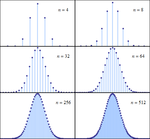


中心極限定理は、ある特定の(かなり一般的な)条件下では、多数のランダム変数の合計がほぼ正規分布に従うと述べています。より具体的には、 は同じ任意分布、ゼロ平均、および分散を持つ独立した同一分布のランダム変数であり、はその平均を でスケールしたものです。 すると、 が増加するにつれて、 の確率分布は、ゼロ平均、分散 の正規分布に近づくようになります。


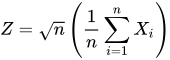
依存度と分布のモーメントに特定の制約が課される場合、定理は独立していない変数や同一に分布していない 変数に拡張できます。

実際に遭遇する多くの検定統計量、スコア、推定量には、特定のランダム変数の合計が含まれており、影響関数を使用することで、さらに多くの推定量をランダム変数の合計として表すことができます。中心極限定理は、これらの統計パラメータが漸近的に正規分布することを意味します。
中心極限定理は、特定の分布が正規分布で近似できることも意味します。たとえば、
- 二項分布は 、平均と分散が大きく、 0 または 1 に近すぎない、ほぼ正規分布です。
- パラメータ のポアソン分布は、の値が大きい場合、平均と分散の正規分布に近似します。[38]
- カイ二乗分布は 、 が大きい場合、平均と分散でほぼ正規分布になります。
- が大きい場合、スチューデントの t 分布は 平均 0、分散 1 でほぼ正規分布になります。


これらの近似値が十分に正確であるかどうかは、近似値が必要とされる目的と、正規分布への収束率によって異なります。通常、このような近似値は分布の末端では精度が低くなります。
中心極限定理における近似誤差の一般的な上限はベリー・エッセン定理によって与えられ、近似の改良はエッジワース展開によって与えられます。
この定理は、多数の均一なノイズ源の合計をガウスノイズとしてモデル化することを正当化するためにも使用できます。AWGN を参照してください。
通常の変数の演算と機能


1つ以上の独立したまたは相関のある正規変数の任意の関数の確率密度、累積分布、逆累積分布は、レイトレーシング[39](Matlabコード)の数値法で計算できます。次のセクションでは、いくつかの特殊なケースを見ていきます。
単一の通常変数に対する操作
が平均と分散で正規分布している場合、
- は、任意の実数およびに対して、平均および分散で正規分布します。つまり、正規分布族は線形変換に対して閉じています。
- の指数は対数正規分布します。
- の標準シグモイドはロジット正規分布します: 。
- の絶対値は折り畳み正規分布に従います。これは半正規分布と呼ばれます。
- 正規化された残差の絶対値 は、自由度 1 のカイ 分布に従います。
- の二乗は、自由度 1 の非心カイ二乗分布に従います。 の場合、分布は単にカイ二乗と呼ばれます。
- 正規変数の対数尤度は、単にその確率密度関数の対数です。これは標準正規変数のスケーリングおよびシフトされた二乗であるため、スケーリングおよびシフトされたカイ二乗変数として分布します。
- 変数をある区間に制限した分布は、切断正規分布と呼ばれます。
- 位置 0 、スケール のレヴィ分布に従います。






2つの独立した正規変数に対する演算
- および が、平均、分散の2 つの独立した正規確率変数である場合、それらの合計も正規分布し、 [証明]平均および分散になります。
- 特に、とが平均0、分散 で独立した正規偏差である場合、ともまた独立しており、平均0、分散 で正規分布します。これは分極恒等式の特別な場合です。[40]
- 、が平均、分散 の2 つの独立した正規偏差であり、、が任意の実数である場合、変数も平均、分散の正規分布になります。したがって、正規分布は安定しています(指数)。
- 、が正規分布である場合、それらの正規化された幾何平均は、およびを伴う正規分布です(視覚化についてはここを参照)。


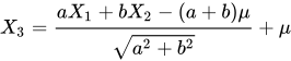


2つの独立した標準正規変数に対する演算
とが平均0、分散1の2つの独立した標準正規分布のランダム変数である 場合、
- それらの和と差は平均 0、分散 2 で正規分布します。
- それらの積は、密度関数 を持つ積分布[41]に従います。ここで、 は第二種修正ベッセル関数です。この分布はゼロの周りで対称で、 で無制限であり、特性関数を持ちます。
- それらの比率は標準のコーシー分布に従います。
- それらのユークリッドノルムはレイリー分布に従います。


複数の独立した正規変数に対する演算
- 独立した正規偏差の任意の線形結合は正規偏差です。
- が独立した標準正規分布に従う場合、それらの平方和は自由度が
- が平均と分散を持つ独立した正規分布するランダム変数である場合、その標本平均は標本標準偏差から独立しており、[42]これはBasuの定理またはCochranの定理を使用して証明できます。[43]これら2つの量の比は、自由度を持つスチューデントのt分布に従います。
- が独立した標準正規分布の確率変数である場合、それらの正規化された平方和の比は自由度が( n , m )のF分布に従う: [44]



![{\displaystyle t={\frac {{\overline {X}}-\mu }{S/{\sqrt {n}}}}={\frac {{\frac {1}{n}}(X_{1}+\cdots +X_{n})-\mu }{\sqrt {{\frac {1}{n(n-1)}}\left[(X_{1}-{\overline {X}})^{2}+\cdots +(X_{n}-{\overline {X}})^{2}\right]}}}\sim t_{n-1}.}](https://wikimedia.org/api/rest_v1/media/math/render/svg/36ff0d3c79a0504e8f259ef99192b825357914d7)


複数の相関正規変数に対する演算
- 正規ベクトルの二次形式、つまり複数の独立したまたは相関した正規変数の二次関数は、一般化されたカイ二乗変数です。

密度関数に対する演算
分割正規分布は、異なる正規分布の密度関数のスケールされたセクションを結合し、密度を再スケールして 1 つに統合するという観点から最も直接的に定義されます。切断正規分布は、単一の密度関数のセクションを再スケールすることによって生成されます。
無限割り算とクラメールの定理
任意の正の整数に対して、平均と分散 を持つ任意の正規分布は、それぞれ平均と分散を持つ独立した正規偏差の合計の分布である。この特性は無限割り切れる可能性と呼ばれる。[45]


逆に、とが独立した確率変数であり、それらの和が正規分布に従う場合、との両方が正規偏差でなければならない。[46]
この結果はクラメールの分解定理として知られており、 2つの分布の畳み込みが正規分布となるのは、両方が正規分布である場合のみであると言うことと同等である。クラメールの定理は、独立した非ガウス変数の線形結合は、正規分布に任意に近づくことはあっても、厳密に正規分布になることは決してないということを意味している。[31]
カッツ・ベルンシュタインの定理
カッツ・ベルンシュタインの定理は、 XとYが独立であり、かつXとYも独立である場合、XとYは必ず正規分布に従うことを述べている。 [47] [48]
より一般的には、が独立した確率変数である場合、2つの異なる線形結合とが独立であることと、すべてが正規分布かつである場合に限ります。ここで、はの分散を表します。[47]


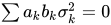

拡張機能
正規分布の概念は、確率論で最も重要な分布の 1 つであり、単変量 (つまり 1 次元) の場合 (ケース 1) の標準的な枠組みをはるかに超えて拡張されています。これらの拡張はすべて正規法則またはガウス法則とも呼ばれるため、名前にはある程度の曖昧さが存在します。
- 多変量正規分布は、k次元ユークリッド空間におけるガウスの法則を記述する。ベクトルX∈Rkは、その成分Σの任意の線形結合が多変量正規分布である場合に多変量正規分布となる。kj =
1a j X j は(一変量)正規分布に従います。 Xの分散は、 k×k対称正定値行列 Vです。 多変量正規分布は、楕円分布の特殊なケースです。そのため、 k = 2 の場合の等密度軌跡は楕円であり、任意のkの場合は楕円体です。 - 修正ガウス分布は、すべての負の要素が 0 にリセットされた正規分布の修正バージョンです。
- 複素正規分布は複素正規ベクトルを扱います。複素ベクトルX ∈ C k は、その実数部と虚数部の両方が 2 k次元の多変量正規分布を持つ場合、正規分布であると言われます。Xの分散共分散構造は、分散行列 Γ と関係行列 Cの 2 つの行列によって記述されます。
- 行列正規分布は、正規分布する行列の場合を説明します。
- ガウス過程は正規分布する確率過程である。これらは、ある無限次元ヒルベルト空間 Hの要素として見ることができるため、 k = ∞の場合の多変量正規ベクトルの類似物である。任意の定数a ∈ Hに対してスカラー積( a , h )が (一変量) 正規分布に従う場合、ランダム要素h ∈ Hは正規であると言われる。このようなガウスランダム要素の分散構造は、線形共分散演算子 K: H → Hで記述できる。いくつかのガウス過程は、独自の名前を持つほど人気になった。
- ガウス q 分布は、正規分布のq 類似物を表す抽象的な数学的構成です。
- q-ガウス分布は、ツァリスエントロピーを最大化するという意味でガウス分布に類似しており、ツァリス分布の一種です。この分布は、上記のガウスq分布とは異なります。
- カニアダキスκ-ガウス分布は、カニアダキス統計から生じるガウス分布の一般化であり、カニアダキス分布の 1 つです。
確率変数Xは、分布が2つの部分からなる正規分布を持つ。


ここで、μ は平均であり、σ 1 2とσ 2 2 はそれぞれ平均の左側と右側の分布の分散です。
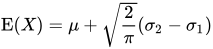
この分布の平均、分散、第三中心モーメントは決定されている[49]

![{\displaystyle \operatorname {T} (X)={\sqrt {\frac {2}{\pi }}}(\sigma _{2}-\sigma _{1})\left[\left({\frac {4}{\pi }}-1\right)(\sigma _{2}-\sigma _{1})^{2}+\sigma _{1}\sigma _{2}\right]}](https://wikimedia.org/api/rest_v1/media/math/render/svg/9959f2c5186e2ed76884054edaf837a602ac6fac)
ここでE( X )、V( X )、T( X )はそれぞれ平均、分散、3次中心モーメントです。
ガウスの法則の主な実用的な用途の 1 つは、実際に遭遇するさまざまなランダム変数の経験的分布をモデル化することです。このような場合、可能な拡張は、2 つ以上のパラメーターを持つより豊富な分布族であり、経験的分布をより正確に適合させることができます。このような拡張の例は次のとおりです。
統計的推論
パラメータの推定
正規分布のパラメータがわからず、代わりに推定したい場合がよくあります。つまり、正規分布の標本からパラメータとのおおよその値を知りたいのです。この問題に対する標準的なアプローチは最大尤度法であり、対数尤度関数を最大化する必要があります。 および について導関数をとり、結果として得られる一階条件系を解くと、最大尤度推定値が得られます。



すると次のようになります。

![{\displaystyle \ln {\mathcal {L}}({\hat {\mu }},{\hat {\sigma }}^{2})=(-n/2)[\ln(2\pi {\hat {\sigma }}^{2})+1]}](https://wikimedia.org/api/rest_v1/media/math/render/svg/561353e6bc80d226fddd9510be61d21bc67b3aee)
サンプル平均
推定量はすべての観測値の算術平均であるため、標本平均と呼ばれます。統計量はに対して完全かつ十分であるため、レーマン・シェッフェの定理により、一様最小分散不偏(UMVU) 推定量となります。 [50]有限標本では、正規分布します。 この推定量の分散は、逆フィッシャー情報行列のμμ要素に等しくなります。これは、推定量が有限標本効率的 であることを意味します。実用上重要なのは、 の標準誤差が に比例するという事実です。つまり、標準誤差を 10 倍に減らしたい場合は、標本内の点の数を 100 倍に増やす必要があります。この事実は、世論調査の標本サイズやモンテカルロシミュレーションの試行回数を決定する際に広く使用されています。





漸近理論の観点からは、は矛盾しません。つまり、 のとき確率的に に収束します。推定量は漸近的に正規でもあります。これは、有限サンプルでは正規であるという事実の単純な帰結です。


サンプル分散
推定量は標本分散と呼ばれます。これは標本 ( ) の分散だからです。実際には、 の代わりに別の推定量がよく使用されます。この別の推定量は と表記され 、標本分散とも呼ばれますが、これは用語の曖昧さを表しています。その平方根は標本標準偏差と呼ばれます。推定量は、分母にnではなく ( n − 1)を持つ点でと異なります(いわゆるベッセル補正)。 と の差は、nが大きい場合は無視できるほど小さくなります。ただし、有限標本では、 を使用する理由は、基礎となるパラメータ の不偏推定量であるのに対し、は偏りがあるからです。また、レーマン・シェッフェの定理により、推定量は一様最小分散不偏 ( UMVU )であり、 [50]すべての不偏推定量の中で「最良」の推定量となります。しかし、平均二乗誤差(MSE) 基準の点では、バイアス推定量の方が よりも優れていることが示されます。有限サンプルでは、 と はどちらも自由度 ( n − 1)の尺度カイ二乗分布に従います。 これらの式の最初のものは、 の分散がに等しく、逆フィッシャー情報行列 のσσ要素よりもわずかに大きいことを示しています。したがって、は の効率的な推定量ではなく、さらに はUMVU であるため、 の有限サンプルの効率的な推定量は存在しないと結論付けることができます。





漸近理論を適用すると、推定量と推定量は両方とも矛盾しません。つまり、サンプル サイズ のときに確率的に に収束します。2 つの推定量は両方とも漸近的に正規です。 特に、両方の推定量は に対して漸近的に効率的です 。

信頼区間
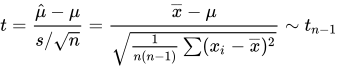
コクランの定理によれば、正規分布の場合、標本平均と標本分散s 2 は独立しており、つまり、それらの結合分布を考慮しても利点はない。逆の定理もある。つまり、標本において標本平均と標本分散が独立している場合、標本は正規分布から来ているに違いない。 とs の間の独立性は、いわゆるt 統計量を構築するために使用できる。
この量tは、自由度( n − 1)のスチューデントの t 分布を持ち、補助統計量(パラメータの値に依存しない) である。このt統計量の分布を反転すると、 μの信頼区間を構築できる。[51]同様に、統計量s 2のχ 2分布を反転すると、 σ 2の信頼区間が得られる。[52]
ここで、t k,pおよびχ
2k
、p はそれぞれt分布とχ 2分布のp番目の分位数です。これらの信頼区間の信頼水準は1 − αです。つまり、真の値μとσ 2 は、確率 (または有意水準) αでこれらの区間から外れます。実際には、通常α = 5%とされ、その結果は 95% 信頼区間となります。σ の信頼区間は、σ 2の区間境界の平方根を取ることで求められます。
![{\displaystyle \mu \in \left[{\hat {\mu }}-{\frac {t_{n-1,1-\alpha /2}}{\sqrt {n}}}s,\,{\hat {\mu }}+{\frac {t_{n-1,1-\alpha /2}}{\sqrt {n}}}s\right],}](https://wikimedia.org/api/rest_v1/media/math/render/svg/1e0b267730af48c4a13b2947e1ee41bd828f92eb)
![{\displaystyle \sigma ^{2}\in \left[{\frac {n-1}{\chi _{n-1,1-\alpha /2}^{2}}}s^{2},\,{\frac {n-1}{\chi _{n-1,\alpha /2}^{2}}}s^{2}\right],}](https://wikimedia.org/api/rest_v1/media/math/render/svg/4a8fc65b99199a5894b71f3089dc1643322dd875)
およびs 2の漸近分布から近似式を導くことができます。 近似式はn の大きな値に対して有効になり、標準正規分布の分位数z α /2 はnに依存しないため、手動計算ではより便利です。特に、最も一般的なα = 5%の値は、 | z 0.025 | = 1.96になります。
![{\displaystyle \mu \in \left[{\hat {\mu }}-{\frac {|z_{\alpha /2}|}{\sqrt {n}}}s,\,{\hat {\mu }}+{\frac {|z_{\alpha /2}|}{\sqrt {n}}}s\right],}](https://wikimedia.org/api/rest_v1/media/math/render/svg/8aeaa29c4240ae0df25b32b05941ea7548e9e4dd)
![{\displaystyle \sigma ^{2}\in \left[s^{2}-{\sqrt {2}}{\frac {|z_{\alpha /2}|}{\sqrt {n}}}s^{2},\,s^{2}+{\sqrt {2}}{\frac {|z_{\alpha /2}|}{\sqrt {n}}}s^{2}\right],}](https://wikimedia.org/api/rest_v1/media/math/render/svg/a019ba33d7f994b3e3bf95f65a69db767894a3cb)
正規性検定
正規性検定は、与えられたデータ セット { x 1 , ..., x n } が正規分布から得られる可能性を評価します。通常、帰無仮説 H 0は、観測値が不特定の平均μと分散σ 2で正規分布しているというものであり、対立仮説H aは分布が任意であるというものです。この問題に対して、多くの検定 (40 種類以上) が考案されています。その中でも特に有名な検定を以下に概説します。
診断プロットは直感的に魅力的ですが、帰無仮説を受け入れるか拒否するかを非公式な人間の判断に依存するため、同時に主観的です。
- Q-Q プロットは、正規確率プロットまたはランクイットプロットとも呼ばれ、データ セットの並べ替えられた値を、標準正規分布の対応する分位数の期待値に対してプロットしたものです。つまり、これは (Φ −1 ( p k ), x ( k ) ) の形式の点のプロットです。ここで、プロットされた点p kはp k = ( k − α )/( n + 1 − 2 α )に等しく、 α は調整定数で、0 から 1 までの値になります。帰無仮説が真である場合、プロットされた点はほぼ直線上に位置するはずです。
- P-P プロット– Q-Q プロットに似ていますが、あまり使用されません。この方法は、点 (Φ( z ( k ) ), p k )をプロットすることから成ります。正規分布データの場合、このプロットは (0, 0) と (1, 1) の間の 45° の線上にあります。

適合度検定:
モーメントベースのテスト:
- ダゴスティーノのK二乗検定
- ジャック・ベラテスト
- シャピロ・ウィルク検定: これは、Q-Q プロットの線の傾きがσであるという事実に基づいています。この検定では、その傾きの最小二乗推定値とサンプル分散の値を比較し、これら 2 つの量が有意に異なる場合は帰無仮説を棄却します。
経験分布関数に基づくテスト:
正規分布のベイズ分析
正規分布データのベイズ分析は、考えられるさまざまな可能性によって複雑になります。
- 平均または分散のいずれか、あるいはどちらも固定量と見なすことができます。
- 分散が不明な場合、分散を直接使用して分析することも、分散の逆数である精度を使用して分析することもできます。精度を使用して式を表現する理由は、ほとんどの場合の分析が簡略化されるためです。
- 単変量と多変量の両方のケースを考慮する必要があります。
- 未知の変数には、共役事前分布または不適切な 事前分布のいずれかが配置される場合があります。
- ベイズ線形回帰では、基本モデルでデータが正規分布していると仮定し、回帰係数に正規事前分布が配置される場合、追加のケースセットが発生します。結果の分析は、独立した同一分布データの基本ケースと同様です。
非線形回帰の場合の式は共役先行論文にまとめられています。
2つの二次方程式の和
スカラー形式
次の補助式は、事後更新方程式を簡素化するのに役立ちます。事後更新方程式は、そうしないとかなり面倒になります。

この式は、平方展開し、x内の項をグループ化し、平方完成することで、 x内の 2 つの二次方程式の和を書き直したものです。いくつかの項に付随する複素定数因子については、次の点に注意してください。
- 係数はyとzの加重平均の形をとります。
- これは、この係数が量aとbの逆数が直接加算される状況から生じるものと考えられることを示しています。したがって、 aとb自体を組み合わせるには、結果を逆数にし、加算し、さらに逆数にして元の単位に戻す必要があります。これはまさに調和平均によって実行される操作の一種であるため、 がaとbの調和平均の半分であることは驚くべきことではありません。


ベクトル形式
同様の式は、2つのベクトル二次方程式の和についても書くことができます。x、y、z が長さkのベクトルで、AとB が対称でサイズの可逆行列である場合、


どこ

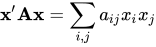
x ′ A x の形式は2次形式と呼ばれ、スカラーです。 言い換えると、 x の要素のペアの積のすべての可能な組み合わせを合計し、それぞれに別々の係数を持ちます。さらに、 であるため、 Aの任意の非対角要素については合計のみが重要であり、 Aが対称であると仮定しても一般性が失われることはありません。さらに、Aが対称である場合、形式


平均からの差の合計
もう一つの便利な式は次の通りです。

既知の差異あり
サイズnのiid正規分布データ ポイントXのセット(各個別のポイントxが既知の分散σ 2に従う) の場合、共役事前分布も正規分布になります。

これは、分散を精度として書き直す、つまり τ = 1/σ 2 を使用することで、より簡単に示すことができます。そして の場合、次のように進めます。


まず、尤度関数は次のようになります (平均からの差の合計については上記の式を使用)。
![{\displaystyle {\begin{aligned}p(\mathbf {X} \mid \mu ,\tau )&=\prod _{i=1}^{n}{\sqrt {\frac {\tau }{2\pi }}}\exp \left(-{\frac {1}{2}}\tau (x_{i}-\mu )^{2}\right)\\&=\left({\frac {\tau }{2\pi }}\right)^{n/2}\exp \left(-{\frac {1}{2}}\tau \sum _{i=1}^{n}(x_{i}-\mu )^{2}\right)\\&=\left({\frac {\tau }{2\pi }}\right)^{n/2}\exp \left[-{\frac {1}{2}}\tau \left(\sum _{i=1}^{n}(x_{i}-{\bar {x}})^{2}+n({\bar {x}}-\mu )^{2}\right)\right].\end{aligned}}}](https://wikimedia.org/api/rest_v1/media/math/render/svg/c2bcd1c34520a24e29b758a0f7427e79e9d8a414)
次に、次のように進めます。
![{\displaystyle {\begin{aligned}p(\mu \mid \mathbf {X} )&\propto p(\mathbf {X} \mid \mu )p(\mu )\\&=\left({\frac {\tau }{2\pi }}\right)^{n/2}\exp \left[-{\frac {1}{2}}\tau \left(\sum _{i=1}^{n}(x_{i}-{\bar {x}})^{2}+n({\bar {x}}-\mu )^{2}\right)\right]{\sqrt {\frac {\tau _{0}}{2\pi }}}\exp \left(-{\frac {1}{2}}\tau _{0}(\mu -\mu _{0})^{2}\right)\\&\propto \exp \left(-{\frac {1}{2}}\left(\tau \left(\sum _{i=1}^{n}(x_{i}-{\bar {x}})^{2}+n({\bar {x}}-\mu )^{2}\right)+\tau _{0}(\mu -\mu _{0})^{2}\right)\right)\\&\propto \exp \left(-{\frac {1}{2}}\left(n\tau ({\bar {x}}-\mu )^{2}+\tau _{0}(\mu -\mu _{0})^{2}\right)\right)\\&=\exp \left(-{\frac {1}{2}}(n\tau +\tau _{0})\left(\mu -{\dfrac {n\tau {\bar {x}}+\tau _{0}\mu _{0}}{n\tau +\tau _{0}}}\right)^{2}+{\frac {n\tau \tau _{0}}{n\tau +\tau _{0}}}({\bar {x}}-\mu _{0})^{2}\right)\\&\propto \exp \left(-{\frac {1}{2}} (n\tau +\tau _{0})\left(\mu -{\dfrac {n\tau {\bar {x}}+\tau _{0}\mu _{0}}{n\tau +\tau _{0}}}\right)^{2}\right)\end{aligned}}}](https://wikimedia.org/api/rest_v1/media/math/render/svg/96e309ead00fbc8603eced5342aa5df534522d6a)
上記の導出では、2つの二次方程式の和に上記の式を使用し、 μを含まない定数因子をすべて除去しました。結果は、平均と精度を持つ正規分布の核、つまり



これは、事前パラメータに関する事後パラメータのベイズ更新方程式のセットとして記述できます。
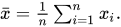
![{\displaystyle {\begin{aligned}\tau _{0}'&=\tau _{0}+n\tau \\[5pt]\mu _{0}'&={\frac {n\tau {\bar {x}}+\tau _{0}\mu _{0}}{n\tau +\tau _{0}}}\\[5pt]{\bar {x}}&={\frac {1}{n}}\sum _{i=1}^{n}x_{i}\end{aligned}}}](https://wikimedia.org/api/rest_v1/media/math/render/svg/a6cfbdf504b1a9ce4cbe79561b4ae983fdf7271d)
つまり、総精度がnτ (または、総分散がn / σ 2 ) で平均値がであるn 個のデータ ポイントを組み合わせるには、データの総精度を事前の総精度に加算するだけで新しい総精度を導き出し、精度加重平均、つまり、それぞれが関連する総精度で重み付けされたデータ平均と事前平均の加重平均によって新しい平均を形成します。精度が観測の確実性を示すものと考えられる場合、これは論理的に意味をなします。事後平均の分布では、各入力コンポーネントがその確実性によって重み付けされ、この分布の確実性は個々の確実性の合計です。(これを直感的に理解するには、「全体が部分の合計よりも大きい (または大きくない)」という表現を比較してください。さらに、事後分布の知識は事前分布と尤度の組み合わせから得られるため、事後分布のほうがそのコンポーネントのいずれよりも確実であると考えるのが理にかなっています。)

上記の式は、正規分布の共役事前分布のベイズ分析を精度の観点から行う方が便利である理由を明らかにしています。事後精度は事前精度と尤度精度の合計であり、事後平均は上記のように精度加重平均によって計算されます。同じ式を分散の観点から書くと、すべての精度を逆数にすることで、より見苦しい式が得られます。
![{\displaystyle {\begin{aligned}{\sigma _{0}^{2}}'&={\frac {1}{{\frac {n}{\sigma ^{2}}}+{\frac {1}{\sigma _{0}^{2}}}}}\\[5pt]\mu _{0}'&={\frac {{\frac {n{\bar {x}}}{\sigma ^{2}}}+{\frac {\mu _{0}}{\sigma _{0}^{2}}}}{{\frac {n}{\sigma ^{2}}}+{\frac {1}{\sigma _{0}^{2}}}}}\\[5pt]{\bar {x}}&={\frac {1}{n}}\sum _{i=1}^{n}x_{i}\end{aligned}}}](https://wikimedia.org/api/rest_v1/media/math/render/svg/ea454c8840683777ce8192d9ae63068c63962858)
平均値がわかっている場合
サイズnのiid正規分布データ ポイントXのセットで、各ポイントx が既知の平均 μ に従う場合、分散の共役事前分布は逆ガンマ分布またはスケール逆カイ 2 乗分布になります。この 2 つは、パラメーター化が異なることを除いて同等です。逆ガンマの方が一般的に使用されますが、便宜上、スケール逆カイ 2 乗を使用します。σ 2の事前分布は次のとおりです。
![{\displaystyle p(\sigma ^{2}\mid \nu _{0},\sigma _{0}^{2})={\frac {(\sigma _{0}^{2}{\frac {\nu _{0}}{2}})^{\nu _{0}/2}}{\Gamma \left({\frac {\nu _{0}}{2}}\right)}}~{\frac {\exp \left[{\frac {-\nu _{0}\sigma _{0}^{2}}{2\sigma ^{2}}}\right]}{(\sigma ^{2})^{1+{\frac {\nu _{0}}{2}}}}}\propto {\frac {\exp \left[{\frac {-\nu _{0}\sigma _{0}^{2}}{2\sigma ^{2}}}\right]}{(\sigma ^{2})^{1+{\frac {\nu _{0}}{2}}}}}}](https://wikimedia.org/api/rest_v1/media/math/render/svg/ef2528fe4774a93087d4adae570ef9ab84707f52)
上記の尤度関数を分散の観点から記述すると、次のようになります。
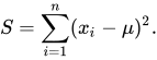
![{\displaystyle {\begin{aligned}p(\mathbf {X} \mid \mu ,\sigma ^{2})&=\left({\frac {1}{2\pi \sigma ^{2}}}\right)^{n/2}\exp \left[-{\frac {1}{2\sigma ^{2}}}\sum _{i=1}^{n}(x_{i}-\mu )^{2}\right]\\&=\left({\frac {1}{2\pi \sigma ^{2}}}\right)^{n/2}\exp \left[-{\frac {S}{2\sigma ^{2}}}\right]\end{aligned}}}](https://wikimedia.org/api/rest_v1/media/math/render/svg/cc06aa31588bba03e4748f8f345f0638a75dc156)
どこ
それから:
![{\displaystyle {\begin{aligned}p(\sigma ^{2}\mid \mathbf {X} )&\propto p(\mathbf {X} \mid \sigma ^{2})p(\sigma ^{2})\\&=\left({\frac {1}{2\pi \sigma ^{2}}}\right)^{n/2}\exp \left[-{\frac {S}{2\sigma ^{2}}}\right]{\frac {(\sigma _{0}^{2}{\frac {\nu _{0}}{2}})^{\frac {\nu _{0}}{2}}}{\Gamma \left({\frac {\nu _{0}}{2}}\right)}}~{\frac {\exp \left[{\frac {-\nu _{0}\sigma _{0}^{2}}{2\sigma ^{2}}}\right]}{(\sigma ^{2})^{1+{\frac {\nu _{0}}{2}}}}}\\&\propto \left({\frac {1}{\sigma ^{2}}}\right)^{n/2}{\frac {1}{(\sigma ^{2})^{1+{\frac {\nu _{0}}{2}}}}}\exp \left[-{\frac {S}{2\sigma ^{2}}}+{\frac {-\nu _{0}\sigma _{0}^{2}}{2\sigma ^{2}}}\right]\\&={\frac {1}{(\sigma ^{2})^{1+{\frac {\nu _{0}+n}{2}}}}}\exp \left[-{\frac {\nu _{0}\sigma _{0}^{2}+S}{2\sigma ^{2}}}\right]\end{aligned}}}](https://wikimedia.org/api/rest_v1/media/math/render/svg/381c1b93f6dc76e2cdca9f3f1f77132dd51dc55f)
上記は、スケール逆カイ二乗分布であり、
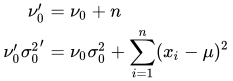
または同等
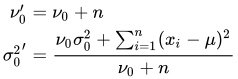
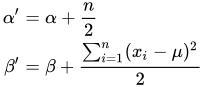
逆ガンマ分布の観点から再パラメータ化すると、結果は次のようになります。
平均値と分散が不明の場合
各点x が未知の平均 μ と未知の分散σ 2に従う、サイズnのiid正規分布データ ポイントXのセットの場合、平均と分散に対して、正規逆ガンマ分布で構成される複合 (多変量)共役事前分布が配置されます。論理的には、これは次のように発生します。
- 平均は不明だが分散は既知のケースの分析から、更新方程式には、データ ポイントの平均と、データ ポイントの合計分散 (既知の分散をデータ ポイントの数で割って計算) で構成されるデータから計算された十分な統計量が含まれることがわかります。
- 分散は不明だが平均はわかっている場合の分析から、更新方程式には、データ ポイントの数と偏差の二乗和で構成されるデータに対する十分な統計量が含まれていることがわかります。
- 事後更新値は、さらにデータを処理する際に事前分布として機能することに注意してください。したがって、可能な限り同じセマンティクスを念頭に置きながら、先ほど説明した十分な統計量の観点から事前分布を論理的に考える必要があります。
- 平均と分散の両方が未知のケースを処理するには、平均、総分散、分散事前分布の計算に使用されるデータ ポイントの数、および偏差の二乗和の固定推定値を使用して、平均と分散に独立した事前分布を配置することができます。ただし、実際には、平均の総分散は未知の分散に依存し、分散事前分布に含まれる偏差の二乗和は未知の平均に依存する (ように見える) ことに注意してください。実際には、後者の依存関係は比較的重要ではありません。実際の平均をシフトすると、生成されたポイントが同じ量だけシフトし、平均すると偏差の二乗は同じままになります。ただし、平均の総分散の場合はそうではありません。未知の分散が増加すると、平均の総分散も比例して増加するため、この依存関係を捉えたいと考えます。
- これは、未知の分散に対する平均の条件付き事前分布を作成し、事前分布に関連付けられた疑似観測の平均を指定するハイパーパラメータと、疑似観測の数を指定する別のパラメータを作成することを示唆しています。この数は分散のスケーリングパラメータとして機能し、実際の分散パラメータに対する平均の全体的な分散を制御できるようにします。分散の事前分布には 2 つのハイパーパラメータもあり、1 つは事前分布に関連付けられた疑似観測の偏差の二乗の合計を指定し、もう 1 つは疑似観測の数を指定します。各事前分布には疑似観測の数を指定するハイパーパラメータがあり、それぞれの場合でその事前分布の相対的な分散を制御します。これらは 2 つの別々のハイパーパラメータとして指定されるため、2 つの事前分布の分散 (信頼度とも呼ばれます) を個別に制御できます。
- これにより、共役事前分布(分散上の逆ガンマ分布と、分散を条件とする平均上の正規分布)が使用され、先ほど定義した同じ 4 つのパラメータを使用して、先ほど定義した 2 つの分布の積である正規逆ガンマ分布が直ちに得られます。
事前確率は通常、次のように定義されます。

更新方程式は次のように導出できます。
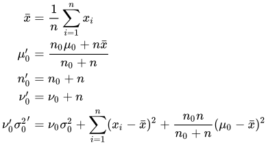
疑似観測値のそれぞれの数に実際の観測値の数が追加されます。新しい平均ハイパーパラメータは再び加重平均ですが、今回は観測値の相対数によって加重されます。最後に、の更新は既知の平均の場合と同様ですが、この場合、偏差の二乗和は真の平均ではなく観測データの平均に対して取られるため、結果として、以前の平均とデータの平均の偏差から生じる追加のエラー ソースに対処するために新しい相互作用項を追加する必要があります。

証拠
事前分布は
![{\displaystyle {\begin{aligned}p(\mu \mid \sigma ^{2};\mu _{0},n_{0})&\sim {\mathcal {N}}(\mu _{0},\sigma ^{2}/n_{0})={\frac {1}{\sqrt {2\pi {\frac {\sigma ^{2}}{n_{0}}}}}}\exp \left(-{\frac {n_{0}}{2\sigma ^{2}}}(\mu -\mu _{0})^{2}\right)\\&\propto (\sigma ^{2})^{-1/2}\exp \left(-{\frac {n_{0}}{2\sigma ^{2}}}(\mu -\mu _{0})^{2}\right)\\p(\sigma ^{2};\nu _{0},\sigma _{0}^{2})&\sim I\chi ^{2}(\nu _{0},\sigma _{0}^{2})=IG(\nu _{0}/2,\nu _{0}\sigma _{0}^{2}/2)\\&={\frac {(\sigma _{0}^{2}\nu _{0}/2)^{\nu _{0}/2}}{\Gamma (\nu _{0}/2)}}~{\frac {\exp \left[{\frac {-\nu _{0}\sigma _{0}^{2}}{2\sigma ^{2}}}\right]}{(\sigma ^{2})^{1+\nu _{0}/2}}}\\&\propto {(\sigma ^{2})^{-(1+\nu _{0}/2)}}\exp \left[{\frac {-\nu _{0}\sigma _{0}^{2}}{2\sigma ^{2}}}\right].\end{aligned}}}](https://wikimedia.org/api/rest_v1/media/math/render/svg/cf7afb8e3b63fb1526171840344b32458e55cf8b)
したがって、結合事前確率は
![{\displaystyle {\begin{aligned}p(\mu ,\sigma ^{2};\mu _{0},n_{0},\nu _{0},\sigma _{0}^{2})&=p(\mu \mid \sigma ^{2};\mu _{0},n_{0})\,p(\sigma ^{2};\nu _{0},\sigma _{0}^{2})\\&\propto (\sigma ^{2})^{-(\nu _{0}+3)/2}\exp \left[-{\frac {1}{2\sigma ^{2}}}\left(\nu _{0}\sigma _{0}^{2}+n_{0}(\mu -\mu _{0})^{2}\right)\right].\end{aligned}}}](https://wikimedia.org/api/rest_v1/media/math/render/svg/b6f808161077baef3854dbfd90b870698d721090)
上記のセクションの既知の分散を持つ 尤度関数は次のようになります。
![{\displaystyle {\begin{aligned}p(\mathbf {X} \mid \mu ,\sigma ^{2})&=\left({\frac {1}{2\pi \sigma ^{2}}}\right)^{n/2}\exp \left[-{\frac {1}{2\sigma ^{2}}}\left(\sum _{i=1}^{n}(x_{i}-\mu )^{2}\right)\right]\end{aligned}}}](https://wikimedia.org/api/rest_v1/media/math/render/svg/f3d77342aadcb34c5d84418cecaefdb52842b6b7)
これを精度ではなく分散で表すと次のようになります 。
![{\displaystyle {\begin{aligned}p(\mathbf {X} \mid \mu ,\sigma ^{2})&=\left({\frac {1}{2\pi \sigma ^{2}}}\right)^{n/2}\exp \left[-{\frac {1}{2\sigma ^{2}}}\left(\sum _{i=1}^{n}(x_{i}-{\bar {x}})^{2}+n({\bar {x}}-\mu )^{2}\right)\right]\\&\propto {\sigma ^{2}}^{-n/2}\exp \left[-{\frac {1}{2\sigma ^{2}}}\left(S+n({\bar {x}}-\mu )^{2}\right)\right]\end{aligned}}}](https://wikimedia.org/api/rest_v1/media/math/render/svg/29b915f070b522a1e9f419be05624c86c854ca14)

したがって、事後分布は次のようになります(条件付け要因としてのハイパーパラメータを除外)。
![{\displaystyle {\begin{aligned}p(\mu ,\sigma ^{2}\mid \mathbf {X} )&\propto p(\mu ,\sigma ^{2})\,p(\mathbf {X} \mid \mu ,\sigma ^{2})\\&\propto (\sigma ^{2})^{-(\nu _{0}+3)/2}\exp \left[-{\frac {1}{2\sigma ^{2}}}\left(\nu _{0}\sigma _{0}^{2}+n_{0}(\mu -\mu _{0})^{2}\right)\right]{\sigma ^{2}}^{-n/2}\exp \left[-{\frac {1}{2\sigma ^{2}}}\left(S+n({\bar {x}}-\mu )^{2}\right)\right]\\&=(\sigma ^{2})^{-(\nu _{0}+n+3)/2}\exp \left[-{\frac {1}{2\sigma ^{2}}}\left(\nu _{0}\sigma _{0}^{2}+S+n_{0}(\mu -\mu _{0})^{2}+n({\bar {x}}-\mu )^{2}\right)\right]\\&=(\sigma ^{2})^{-(\nu _{0}+n+3)/2}\exp \left[-{\frac {1}{2\sigma ^{2}}}\left(\nu _{0}\sigma _{0}^{2}+S+{\frac {n_{0}n}{n_{0}+n}}(\mu _{0}-{\bar {x}})^{2}+(n_{0}+n)\left(\mu -{\frac {n_{0}\mu _{0}+n{\bar {x}}}{n_{0}+n}}\right)^{2}\right)\right]\\&\propto (\sigma ^{2})^{-1/2}\exp \left[-{\frac {n_{0}+n}{2\sigma ^{2}}}\left(\mu -{\frac {n_{0}\mu _{0}+n{\bar {x}}}{n_{0}+n}}\right)^{2}\right]\\&\quad \times (\sigma ^{2})^{-(\nu _{0}/2+n/2+1)}\exp \left[-{\frac {1}{2\sigma ^{2}}}\left(\nu _{0}\sigma _{0}^{2}+S+{\frac {n_{0}n}{n_{0}+n}}(\mu _{0}-{\bar {x}})^{2}\right)\right]\\&={\mathcal {N}}_{\mu \mid \sigma ^{2}}\left({\frac {n_{0}\mu _{0}+n{\bar {x}}}{n_{0}+n}},{\frac {\sigma ^{2}}{n_{0}+n}}\right)\cdot {\rm {IG}}_{\sigma ^{2}}\left({\frac {1}{2}}(\nu _{0}+n),{\frac {1}{2}}\left(\nu _{0}\sigma _{0}^{2}+S+{\frac {n_{0}n}{n_{0}+n}}(\mu _{0}-{\bar {x}})^{2}\right)\right).\end{aligned}}}](https://wikimedia.org/api/rest_v1/media/math/render/svg/cad9489034d77d53c12c7ee6044f712cfdb77831)
言い換えると、事後分布は、 上の正規分布と上の逆ガンマ分布の積の形を持ち、パラメータは上記の更新方程式と同じです。


発生と応用
実際の問題における正規分布の発生は、大まかに次の 4 つのカテゴリに分類できます。
- 正確には正規分布です。
- 近似正規法則、例えば、そのような近似が中心極限定理によって正当化される場合、および
- Distributions modeled as normal – the normal distribution being the distribution with maximum entropy for a given mean and variance.
- Regression problems – the normal distribution being found after systematic effects have been modeled sufficiently well.
Exact normality
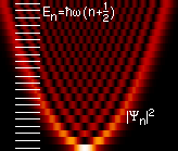
Certain quantities in physics are distributed normally, as was first demonstrated by James Clerk Maxwell. Examples of such quantities are:
- Probability density function of a ground state in a quantum harmonic oscillator.
- The position of a particle that experiences diffusion. If initially the particle is located at a specific point (that is its probability distribution is the Dirac delta function), then after time t its location is described by a normal distribution with variance t, which satisfies the diffusion equation . If the initial location is given by a certain density function , then the density at time t is the convolution of g and the normal probability density function.


Approximate normality
Approximately normal distributions occur in many situations, as explained by the central limit theorem. When the outcome is produced by many small effects acting additively and independently, its distribution will be close to normal. The normal approximation will not be valid if the effects act multiplicatively (instead of additively), or if there is a single external influence that has a considerably larger magnitude than the rest of the effects.
- In counting problems, where the central limit theorem includes a discrete-to-continuum approximation and where infinitely divisible and decomposable distributions are involved, such as
- Binomial random variables, associated with binary response variables;
- Poisson random variables, associated with rare events;
- Thermal radiation has a Bose–Einstein distribution on very short time scales, and a normal distribution on longer timescales due to the central limit theorem.
Assumed normality

I can only recognize the occurrence of the normal curve – the Laplacian curve of errors – as a very abnormal phenomenon. It is roughly approximated to in certain distributions; for this reason, and on account for its beautiful simplicity, we may, perhaps, use it as a first approximation, particularly in theoretical investigations.
— Pearson (1901)
There are statistical methods to empirically test that assumption; see the above Normality tests section.
- In biology, the logarithm of various variables tend to have a normal distribution, that is, they tend to have a log-normal distribution (after separation on male/female subpopulations), with examples including:
- Measures of size of living tissue (length, height, skin area, weight);[53]
- The length of inert appendages (hair, claws, nails, teeth) of biological specimens, in the direction of growth; presumably the thickness of tree bark also falls under this category;
- Certain physiological measurements, such as blood pressure of adult humans.
- In finance, in particular the Black–Scholes model, changes in the logarithm of exchange rates, price indices, and stock market indices are assumed normal (these variables behave like compound interest, not like simple interest, and so are multiplicative). Some mathematicians such as Benoit Mandelbrot have argued that log-Levy distributions, which possesses heavy tails would be a more appropriate model, in particular for the analysis for stock market crashes. The use of the assumption of normal distribution occurring in financial models has also been criticized by Nassim Nicholas Taleb in his works.
- Measurement errors in physical experiments are often modeled by a normal distribution. This use of a normal distribution does not imply that one is assuming the measurement errors are normally distributed, rather using the normal distribution produces the most conservative predictions possible given only knowledge about the mean and variance of the errors.[54]
- In standardized testing, results can be made to have a normal distribution by either selecting the number and difficulty of questions (as in the IQ test) or transforming the raw test scores into output scores by fitting them to the normal distribution. For example, the SAT's traditional range of 200–800 is based on a normal distribution with a mean of 500 and a standard deviation of 100.
- Many scores are derived from the normal distribution, including percentile ranks (percentiles or quantiles), normal curve equivalents, stanines, z-scores, and T-scores. Additionally, some behavioral statistical procedures assume that scores are normally distributed; for example, t-tests and ANOVAs. Bell curve grading assigns relative grades based on a normal distribution of scores.
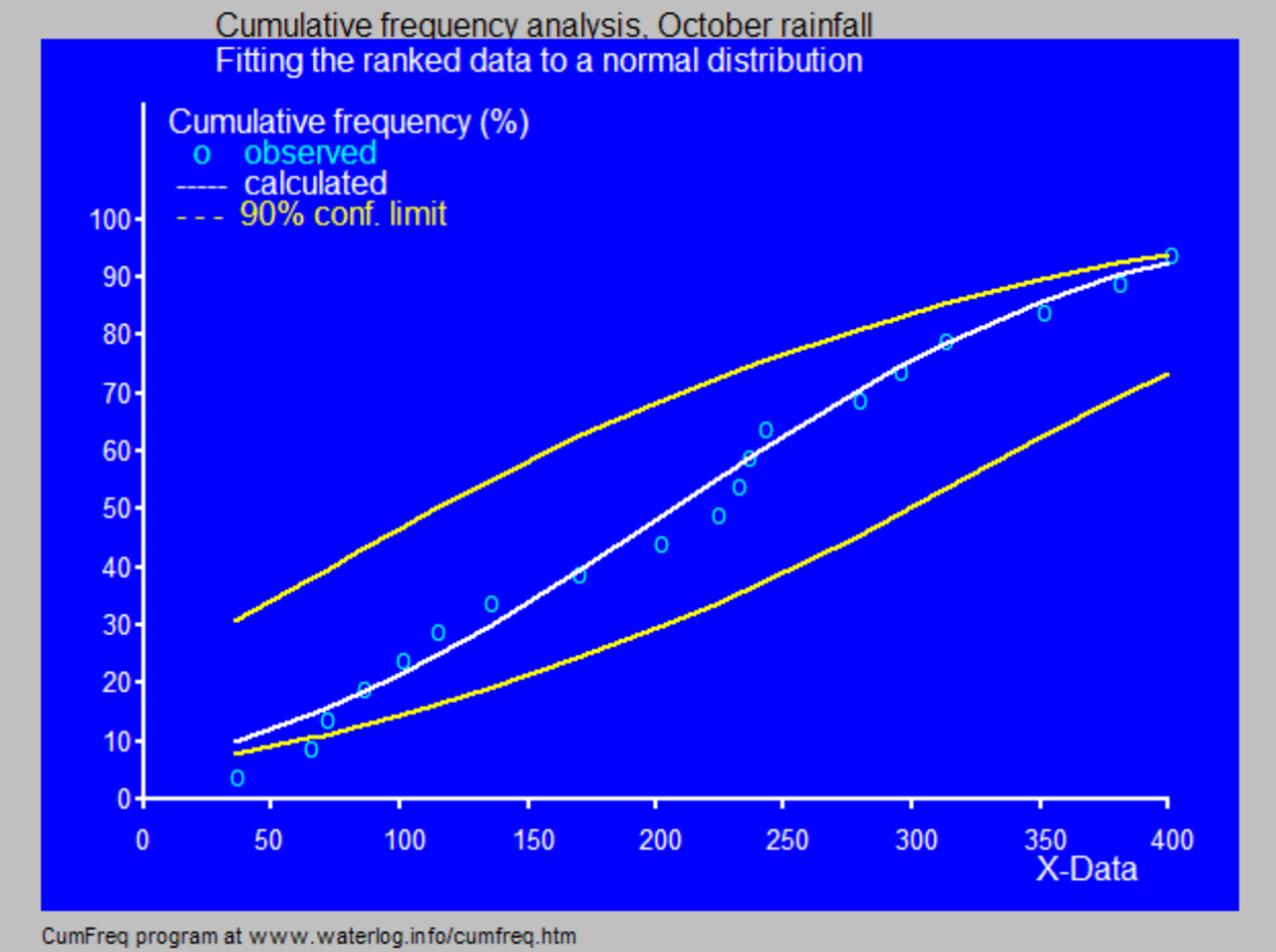
- In hydrology the distribution of long duration river discharge or rainfall, e.g. monthly and yearly totals, is often thought to be practically normal according to the central limit theorem.[55] The blue picture, made with CumFreq, illustrates an example of fitting the normal distribution to ranked October rainfalls showing the 90% confidence belt based on the binomial distribution. The rainfall data are represented by plotting positions as part of the cumulative frequency analysis.
Methodological problems and peer review
John Ioannidis argued that using normally distributed standard deviations as standards for validating research findings leave falsifiable predictions about phenomena that are not normally distributed untested. This includes, for example, phenomena that only appear when all necessary conditions are present and one cannot be a substitute for another in an addition-like way and phenomena that are not randomly distributed. Ioannidis argues that standard deviation-centered validation gives a false appearance of validity to hypotheses and theories where some but not all falsifiable predictions are normally distributed since the portion of falsifiable predictions that there is evidence against may and in some cases are in the non-normally distributed parts of the range of falsifiable predictions, as well as baselessly dismissing hypotheses for which none of the falsifiable predictions are normally distributed as if were they unfalsifiable when in fact they do make falsifiable predictions. It is argued by Ioannidis that many cases of mutually exclusive theories being accepted as validated by research journals are caused by failure of the journals to take in empirical falsifications of non-normally distributed predictions, and not because mutually exclusive theories are true, which they cannot be, although two mutually exclusive theories can both be wrong and a third one correct.[56]
Computational methods
Generating values from normal distribution
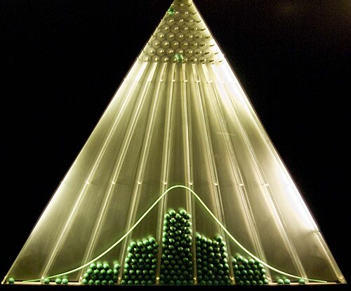
In computer simulations, especially in applications of the Monte-Carlo method, it is often desirable to generate values that are normally distributed. The algorithms listed below all generate the standard normal deviates, since a N(μ, σ2) can be generated as X = μ + σZ, where Z is standard normal. All these algorithms rely on the availability of a random number generator U capable of producing uniform random variates.
- The most straightforward method is based on the probability integral transform property: if U is distributed uniformly on (0,1), then Φ−1(U) will have the standard normal distribution. The drawback of this method is that it relies on calculation of the probit function Φ−1, which cannot be done analytically. Some approximate methods are described in Hart (1968) and in the erf article. Wichura gives a fast algorithm for computing this function to 16 decimal places,[57] which is used by R to compute random variates of the normal distribution.
- An easy-to-program approximate approach that relies on the central limit theorem is as follows: generate 12 uniform U(0,1) deviates, add them all up, and subtract 6 – the resulting random variable will have approximately standard normal distribution. In truth, the distribution will be Irwin–Hall, which is a 12-section eleventh-order polynomial approximation to the normal distribution. This random deviate will have a limited range of (−6, 6).[58] Note that in a true normal distribution, only 0.00034% of all samples will fall outside ±6σ.
- The Box–Muller method uses two independent random numbers U and V distributed uniformly on (0,1). Then the two random variables X and Y will both have the standard normal distribution, and will be independent. This formulation arises because for a bivariate normal random vector (X, Y) the squared norm X2 + Y2 will have the chi-squared distribution with two degrees of freedom, which is an easily generated exponential random variable corresponding to the quantity −2 ln(U) in these equations; and the angle is distributed uniformly around the circle, chosen by the random variable V.
- The Marsaglia polar method is a modification of the Box–Muller method which does not require computation of the sine and cosine functions. In this method, U and V are drawn from the uniform (−1,1) distribution, and then S = U2 + V2 is computed. If S is greater or equal to 1, then the method starts over, otherwise the two quantities are returned. Again, X and Y are independent, standard normal random variables.
- The Ratio method[59] is a rejection method. The algorithm proceeds as follows:
- Generate two independent uniform deviates U and V;
- Compute X = √8/e (V − 0.5)/U;
- Optional: if X2 ≤ 5 − 4e1/4U then accept X and terminate algorithm;
- Optional: if X2 ≥ 4e−1.35/U + 1.4 then reject X and start over from step 1;
- If X2 ≤ −4 lnU then accept X, otherwise start over the algorithm.
- The two optional steps allow the evaluation of the logarithm in the last step to be avoided in most cases. These steps can be greatly improved[60] so that the logarithm is rarely evaluated.
- The ziggurat algorithm[61] is faster than the Box–Muller transform and still exact. In about 97% of all cases it uses only two random numbers, one random integer and one random uniform, one multiplication and an if-test. Only in 3% of the cases, where the combination of those two falls outside the "core of the ziggurat" (a kind of rejection sampling using logarithms), do exponentials and more uniform random numbers have to be employed.
- Integer arithmetic can be used to sample from the standard normal distribution.[62] This method is exact in the sense that it satisfies the conditions of ideal approximation;[63] i.e., it is equivalent to sampling a real number from the standard normal distribution and rounding this to the nearest representable floating point number.
- There is also some investigation[64] into the connection between the fast Hadamard transform and the normal distribution, since the transform employs just addition and subtraction and by the central limit theorem random numbers from almost any distribution will be transformed into the normal distribution. In this regard a series of Hadamard transforms can be combined with random permutations to turn arbitrary data sets into a normally distributed data.


Numerical approximations for the normal cumulative distribution function and normal quantile function
The standard normal cumulative distribution function is widely used in scientific and statistical computing.
The values Φ(x) may be approximated very accurately by a variety of methods, such as numerical integration, Taylor series, asymptotic series and continued fractions. Different approximations are used depending on the desired level of accuracy.
- Zelen & Severo (1964) give the approximation for Φ(x) for x > 0 with the absolute error |ε(x)| < 7.5·10−8 (algorithm 26.2.17): where ϕ(x) is the standard normal probability density function, and b0 = 0.2316419, b1 = 0.319381530, b2 = −0.356563782, b3 = 1.781477937, b4 = −1.821255978, b5 = 1.330274429.
- Hart (1968) lists some dozens of approximations – by means of rational functions, with or without exponentials – for the erfc() function. His algorithms vary in the degree of complexity and the resulting precision, with maximum absolute precision of 24 digits. An algorithm by West (2009) combines Hart's algorithm 5666 with a continued fraction approximation in the tail to provide a fast computation algorithm with a 16-digit precision.
- Cody (1969) after recalling Hart68 solution is not suited for erf, gives a solution for both erf and erfc, with maximal relative error bound, via Rational Chebyshev Approximation.
- Marsaglia (2004) suggested a simple algorithm[note 1] based on the Taylor series expansion for calculating Φ(x) with arbitrary precision. The drawback of this algorithm is comparatively slow calculation time (for example it takes over 300 iterations to calculate the function with 16 digits of precision when x = 10).
- The GNU Scientific Library calculates values of the standard normal cumulative distribution function using Hart's algorithms and approximations with Chebyshev polynomials.
- Dia (2023) proposes the following approximation of with a maximum relative error less than in absolute value: for and for ,







Shore (1982) introduced simple approximations that may be incorporated in stochastic optimization models of engineering and operations research, like reliability engineering and inventory analysis. Denoting p = Φ(z), the simplest approximation for the quantile function is:
![{\displaystyle z=\Phi ^{-1}(p)=5.5556\left[1-\left({\frac {1-p}{p}}\right)^{0.1186}\right],\qquad p\geq 1/2}](https://wikimedia.org/api/rest_v1/media/math/render/svg/5f2df7f1427d0c90d075faef38f4f5ab7acce5c9)
This approximation delivers for z a maximum absolute error of 0.026 (for 0.5 ≤ p ≤ 0.9999, corresponding to 0 ≤ z ≤ 3.719). For p < 1/2 replace p by 1 − p and change sign. Another approximation, somewhat less accurate, is the single-parameter approximation:
![{\displaystyle z=-0.4115\left\{{\frac {1-p}{p}}+\log \left[{\frac {1-p}{p}}\right]-1\right\},\qquad p\geq 1/2}](https://wikimedia.org/api/rest_v1/media/math/render/svg/e1edea9f990058f741db6735799c8b40999b833b)
The latter had served to derive a simple approximation for the loss integral of the normal distribution, defined by
![{\displaystyle {\begin{aligned}L(z)&=\int _{z}^{\infty }(u-z)\varphi (u)\,du=\int _{z}^{\infty }[1-\Phi (u)]\,du\\[5pt]L(z)&\approx {\begin{cases}0.4115\left({\dfrac {p}{1-p}}\right)-z,&p<1/2,\\\\0.4115\left({\dfrac {1-p}{p}}\right),&p\geq 1/2.\end{cases}}\\[5pt]{\text{or, equivalently,}}\\L(z)&\approx {\begin{cases}0.4115\left\{1-\log \left[{\frac {p}{1-p}}\right]\right\},&p<1/2,\\\\0.4115{\dfrac {1-p}{p}},&p\geq 1/2.\end{cases}}\end{aligned}}}](https://wikimedia.org/api/rest_v1/media/math/render/svg/e4b69fa586cffdfbbd40a94c65629726e4ae78bf)
This approximation is particularly accurate for the right far-tail (maximum error of 10−3 for z≥1.4). Highly accurate approximations for the cumulative distribution function, based on Response Modeling Methodology (RMM, Shore, 2011, 2012), are shown in Shore (2005).
Some more approximations can be found at: Error function#Approximation with elementary functions. In particular, small relative error on the whole domain for the cumulative distribution function and the quantile function as well, is achieved via an explicitly invertible formula by Sergei Winitzki in 2008.

History
Development
Some authors[65][66] attribute the credit for the discovery of the normal distribution to de Moivre, who in 1738[note 2] published in the second edition of his The Doctrine of Chances the study of the coefficients in the binomial expansion of (a + b)n. De Moivre proved that the middle term in this expansion has the approximate magnitude of , and that "If m or 1/2n be a Quantity infinitely great, then the Logarithm of the Ratio, which a Term distant from the middle by the Interval ℓ, has to the middle Term, is ."[67] Although this theorem can be interpreted as the first obscure expression for the normal probability law, Stigler points out that de Moivre himself did not interpret his results as anything more than the approximate rule for the binomial coefficients, and in particular de Moivre lacked the concept of the probability density function.[68]


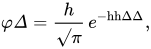
In 1823 Gauss published his monograph "Theoria combinationis observationum erroribus minimis obnoxiae" where among other things he introduces several important statistical concepts, such as the method of least squares, the method of maximum likelihood, and the normal distribution. Gauss used M, M′, M′′, ... to denote the measurements of some unknown quantity V, and sought the most probable estimator of that quantity: the one that maximizes the probability φ(M − V) · φ(M′ − V) · φ(M′′ − V) · ... of obtaining the observed experimental results. In his notation φΔ is the probability density function of the measurement errors of magnitude Δ. Not knowing what the function φ is, Gauss requires that his method should reduce to the well-known answer: the arithmetic mean of the measured values.[note 3] Starting from these principles, Gauss demonstrates that the only law that rationalizes the choice of arithmetic mean as an estimator of the location parameter, is the normal law of errors:[69] where h is "the measure of the precision of the observations". Using this normal law as a generic model for errors in the experiments, Gauss formulates what is now known as the non-linear weighted least squares method.[70]

Although Gauss was the first to suggest the normal distribution law, Laplace made significant contributions.[note 4] It was Laplace who first posed the problem of aggregating several observations in 1774,[71] although his own solution led to the Laplacian distribution. It was Laplace who first calculated the value of the integral ∫ e−t2 dt = √π in 1782, providing the normalization constant for the normal distribution.[72] Finally, it was Laplace who in 1810 proved and presented to the academy the fundamental central limit theorem, which emphasized the theoretical importance of the normal distribution.[73]
It is of interest to note that in 1809 an Irish-American mathematician Robert Adrain published two insightful but flawed derivations of the normal probability law, simultaneously and independently from Gauss.[74] His works remained largely unnoticed by the scientific community, until in 1871 they were exhumed by Abbe.[75]
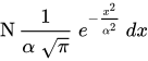
In the middle of the 19th century Maxwell demonstrated that the normal distribution is not just a convenient mathematical tool, but may also occur in natural phenomena:[76] The number of particles whose velocity, resolved in a certain direction, lies between x and x + dx is
Naming
Today, the concept is usually known in English as the normal distribution or Gaussian distribution. Other less common names include Gauss distribution, Laplace-Gauss distribution, the law of error, the law of facility of errors, Laplace's second law, and Gaussian law.
Gauss himself apparently coined the term with reference to the "normal equations" involved in its applications, with normal having its technical meaning of orthogonal rather than usual.[77] However, by the end of the 19th century some authors[note 5] had started using the name normal distribution, where the word "normal" was used as an adjective – the term now being seen as a reflection of the fact that this distribution was seen as typical, common – and thus normal. Peirce (one of those authors) once defined "normal" thus: "...the 'normal' is not the average (or any other kind of mean) of what actually occurs, but of what would, in the long run, occur under certain circumstances."[78] Around the turn of the 20th century Pearson popularized the term normal as a designation for this distribution.[79]
Many years ago I called the Laplace–Gaussian curve the normal curve, which name, while it avoids an international question of priority, has the disadvantage of leading people to believe that all other distributions of frequency are in one sense or another 'abnormal'.
— Pearson (1920)
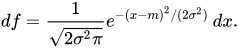
Also, it was Pearson who first wrote the distribution in terms of the standard deviation σ as in modern notation. Soon after this, in year 1915, Fisher added the location parameter to the formula for normal distribution, expressing it in the way it is written nowadays:
The term "standard normal", which denotes the normal distribution with zero mean and unit variance came into general use around the 1950s, appearing in the popular textbooks by P. G. Hoel (1947) Introduction to Mathematical Statistics and A. M. Mood (1950) Introduction to the Theory of Statistics.[80]
See also

- Bates distribution – similar to the Irwin–Hall distribution, but rescaled back into the 0 to 1 range
- Behrens–Fisher problem – the long-standing problem of testing whether two normal samples with different variances have same means;
- Bhattacharyya distance – method used to separate mixtures of normal distributions
- Erdős–Kac theorem – on the occurrence of the normal distribution in number theory
- Full width at half maximum
- Gaussian blur – convolution, which uses the normal distribution as a kernel
- Modified half-normal distribution[81] with the pdf on is given as , where denotes the Fox–Wright Psi function.
- Normally distributed and uncorrelated does not imply independent
- Ratio normal distribution
- Reciprocal normal distribution
- Standard normal table
- Stein's lemma
- Sub-Gaussian distribution
- Sum of normally distributed random variables
- Tweedie distribution – The normal distribution is a member of the family of Tweedie exponential dispersion models.
- Wrapped normal distribution – the Normal distribution applied to a circular domain
- Z-test – using the normal distribution


Notes
- ^ For example, this algorithm is given in the article Bc programming language.
- ^ De Moivre first published his findings in 1733, in a pamphlet Approximatio ad Summam Terminorum Binomii (a + b)n in Seriem Expansi that was designated for private circulation only. But it was not until the year 1738 that he made his results publicly available. The original pamphlet was reprinted several times, see for example Walker (1985).
- ^ "It has been customary certainly to regard as an axiom the hypothesis that if any quantity has been determined by several direct observations, made under the same circumstances and with equal care, the arithmetical mean of the observed values affords the most probable value, if not rigorously, yet very nearly at least, so that it is always most safe to adhere to it." — Gauss (1809, section 177)
- ^ "My custom of terming the curve the Gauss–Laplacian or normal curve saves us from proportioning the merit of discovery between the two great astronomer mathematicians." quote from Pearson (1905, p. 189)
- ^ Besides those specifically referenced here, such use is encountered in the works of Peirce, Galton (Galton (1889, chapter V)) and Lexis (Lexis (1878), Rohrbasser & Véron (2003)) c. 1875.[citation needed]
References
Citations
- ^ Norton, Matthew; Khokhlov, Valentyn; Uryasev, Stan (2019). "Calculating CVaR and bPOE for common probability distributions with application to portfolio optimization and density estimation" (PDF). Annals of Operations Research. 299 (1–2). Springer: 1281–1315. arXiv:1811.11301. doi:10.1007/s10479-019-03373-1. S2CID 254231768. Retrieved February 27, 2023.
- ^ Normal Distribution, Gale Encyclopedia of Psychology
- ^ Casella & Berger (2001, p. 102)
- ^ Lyon, A. (2014). Why are Normal Distributions Normal?, The British Journal for the Philosophy of Science.
- ^ Jorge, Nocedal; Stephan, J. Wright (2006). Numerical Optimization (2nd ed.). Springer. p. 249. ISBN 978-0387-30303-1.
- ^ a b "Normal Distribution". www.mathsisfun.com. Retrieved August 15, 2020.
- ^ Stigler (1982)
- ^ Halperin, Hartley & Hoel (1965, item 7)
- ^ McPherson (1990, p. 110)
- ^ Bernardo & Smith (2000, p. 121)
- ^ Scott, Clayton; Nowak, Robert (August 7, 2003). "The Q-function". Connexions.
- ^ Barak, Ohad (April 6, 2006). "Q Function and Error Function" (PDF). Tel Aviv University. Archived from the original (PDF) on March 25, 2009.
- ^ Weisstein, Eric W. "Normal Distribution Function". MathWorld.
- ^ Abramowitz, Milton; Stegun, Irene Ann, eds. (1983) [June 1964]. "Chapter 26, eqn 26.2.12". Handbook of Mathematical Functions with Formulas, Graphs, and Mathematical Tables. Applied Mathematics Series. Vol. 55 (Ninth reprint with additional corrections of tenth original printing with corrections (December 1972); first ed.). Washington D.C.; New York: United States Department of Commerce, National Bureau of Standards; Dover Publications. p. 932. ISBN 978-0-486-61272-0. LCCN 64-60036. MR 0167642. LCCN 65-12253.
- ^ Vaart, A. W. van der (October 13, 1998). Asymptotic Statistics. Cambridge University Press. doi:10.1017/cbo9780511802256. ISBN 978-0-511-80225-6.
- ^ Cover, Thomas M.; Thomas, Joy A. (2006). Elements of Information Theory. John Wiley and Sons. p. 254. ISBN 9780471748816.
- ^ Park, Sung Y.; Bera, Anil K. (2009). "Maximum Entropy Autoregressive Conditional Heteroskedasticity Model" (PDF). Journal of Econometrics. 150 (2): 219–230. CiteSeerX 10.1.1.511.9750. doi:10.1016/j.jeconom.2008.12.014. Archived from the original (PDF) on March 7, 2016. Retrieved June 2, 2011.
- ^ Geary RC(1936) The distribution of the "Student's ratio for the non-normal samples". Supplement to the Journal of the Royal Statistical Society 3 (2): 178–184
- ^ Lukacs, Eugene (March 1942). "A Characterization of the Normal Distribution". Annals of Mathematical Statistics. 13 (1): 91–93. doi:10.1214/AOMS/1177731647. ISSN 0003-4851. JSTOR 2236166. MR 0006626. Zbl 0060.28509. Wikidata Q55897617.
- ^ a b c Patel & Read (1996, [2.1.4])
- ^ Fan (1991, p. 1258)
- ^ Patel & Read (1996, [2.1.8])
- ^ Papoulis, Athanasios. Probability, Random Variables and Stochastic Processes (4th ed.). p. 148.
- ^ Winkelbauer, Andreas (2012). "Moments and Absolute Moments of the Normal Distribution". arXiv:1209.4340 [math.ST].
- ^ Bryc (1995, p. 23)
- ^ Bryc (1995, p. 24)
- ^ Cover & Thomas (2006, p. 254)
- ^ Williams, David (2001). Weighing the odds : a course in probability and statistics (Reprinted. ed.). Cambridge [u.a.]: Cambridge Univ. Press. pp. 197–199. ISBN 978-0-521-00618-7.
- ^ Smith, José M. Bernardo; Adrian F. M. (2000). Bayesian theory (Reprint ed.). Chichester [u.a.]: Wiley. pp. 209, 366. ISBN 978-0-471-49464-5.
{{cite book}}: CS1 maint: multiple names: authors list (link) - ^ O'Hagan, A. (1994) Kendall's Advanced Theory of statistics, Vol 2B, Bayesian Inference, Edward Arnold. ISBN 0-340-52922-9 (Section 5.40)
- ^ a b Bryc (1995, p. 35)
- ^ UIUC, Lecture 21. The Multivariate Normal Distribution, 21.6:"Individually Gaussian Versus Jointly Gaussian".
- ^ Edward L. Melnick and Aaron Tenenbein, "Misspecifications of the Normal Distribution", The American Statistician, volume 36, number 4 November 1982, pages 372–373
- ^ "Kullback Leibler (KL) Distance of Two Normal (Gaussian) Probability Distributions". Allisons.org. December 5, 2007. Retrieved March 3, 2017.
- ^ Jordan, Michael I. (February 8, 2010). "Stat260: Bayesian Modeling and Inference: The Conjugate Prior for the Normal Distribution" (PDF).
- ^ Amari & Nagaoka (2000)
- ^ "Expectation of the maximum of gaussian random variables". Mathematics Stack Exchange. Retrieved April 7, 2024.
- ^ "Normal Approximation to Poisson Distribution". Stat.ucla.edu. Retrieved March 3, 2017.
- ^ a b Das, Abhranil (2021). "A method to integrate and classify normal distributions". Journal of Vision. 21 (10): 1. arXiv:2012.14331. doi:10.1167/jov.21.10.1. PMC 8419883. PMID 34468706.
- ^ Bryc (1995, p. 27)
- ^ Weisstein, Eric W. "Normal Product Distribution". MathWorld. wolfram.com.
- ^ Lukacs, Eugene (1942). "A Characterization of the Normal Distribution". The Annals of Mathematical Statistics. 13 (1): 91–3. doi:10.1214/aoms/1177731647. ISSN 0003-4851. JSTOR 2236166.
- ^ Basu, D.; Laha, R. G. (1954). "On Some Characterizations of the Normal Distribution". Sankhyā. 13 (4): 359–62. ISSN 0036-4452. JSTOR 25048183.
- ^ Lehmann, E. L. (1997). Testing Statistical Hypotheses (2nd ed.). Springer. p. 199. ISBN 978-0-387-94919-2.
- ^ Patel & Read (1996, [2.3.6])
- ^ Galambos & Simonelli (2004, Theorem 3.5)
- ^ a b Lukacs & King (1954)
- ^ Quine, M.P. (1993). "On three characterisations of the normal distribution". Probability and Mathematical Statistics. 14 (2): 257–263.
- ^ John, S (1982). "The three parameter two-piece normal family of distributions and its fitting". Communications in Statistics – Theory and Methods. 11 (8): 879–885. doi:10.1080/03610928208828279.
- ^ a b Krishnamoorthy (2006, p. 127)
- ^ Krishnamoorthy (2006, p. 130)
- ^ Krishnamoorthy (2006, p. 133)
- ^ Huxley (1932)
- ^ Jaynes, Edwin T. (2003). Probability Theory: The Logic of Science. Cambridge University Press. pp. 592–593. ISBN 9780521592710.
- ^ Oosterbaan, Roland J. (1994). "Chapter 6: Frequency and Regression Analysis of Hydrologic Data" (PDF). In Ritzema, Henk P. (ed.). Drainage Principles and Applications, Publication 16 (second revised ed.). Wageningen, The Netherlands: International Institute for Land Reclamation and Improvement (ILRI). pp. 175–224. ISBN 978-90-70754-33-4.
- ^ Why Most Published Research Findings Are False, John P. A. Ioannidis, 2005
- ^ Wichura, Michael J. (1988). "Algorithm AS241: The Percentage Points of the Normal Distribution". Applied Statistics. 37 (3): 477–84. doi:10.2307/2347330. JSTOR 2347330.
- ^ Johnson, Kotz & Balakrishnan (1995, Equation (26.48))
- ^ Kinderman & Monahan (1977)
- ^ Leva (1992)
- ^ Marsaglia & Tsang (2000)
- ^ Karney (2016)
- ^ Monahan (1985, section 2)
- ^ Wallace (1996)
- ^ Johnson, Kotz & Balakrishnan (1994, p. 85)
- ^ Le Cam & Lo Yang (2000, p. 74)
- ^ De Moivre, Abraham (1733), Corollary I – see Walker (1985, p. 77)
- ^ Stigler (1986, p. 76)
- ^ Gauss (1809, section 177)
- ^ Gauss (1809, section 179)
- ^ Laplace (1774, Problem III)
- ^ Pearson (1905, p. 189)
- ^ Stigler (1986, p. 144)
- ^ Stigler (1978, p. 243)
- ^ Stigler (1978, p. 244)
- ^ Maxwell (1860, p. 23)
- ^ Jaynes, Edwin J.; Probability Theory: The Logic of Science, Ch. 7.
- ^ Peirce, Charles S. (c. 1909 MS), Collected Papers v. 6, paragraph 327.
- ^ Kruskal & Stigler (1997).
- ^ "Earliest Uses... (Entry Standard Normal Curve)".
- ^ Sun, Jingchao; Kong, Maiying; Pal, Subhadip (June 22, 2021). "The Modified-Half-Normal distribution: Properties and an efficient sampling scheme". Communications in Statistics – Theory and Methods. 52 (5): 1591–1613. doi:10.1080/03610926.2021.1934700. ISSN 0361-0926. S2CID 237919587.
Sources
- Aldrich, John; Miller, Jeff. "Earliest Uses of Symbols in Probability and Statistics".
- Aldrich, John; Miller, Jeff. "Earliest Known Uses of Some of the Words of Mathematics". In particular, the entries for "bell-shaped and bell curve", "normal (distribution)", "Gaussian", and "Error, law of error, theory of errors, etc.".
- Amari, Shun-ichi; Nagaoka, Hiroshi (2000). Methods of Information Geometry. Oxford University Press. ISBN 978-0-8218-0531-2.
- Bernardo, José M.; Smith, Adrian F. M. (2000). Bayesian Theory. Wiley. ISBN 978-0-471-49464-5.
- Bryc, Wlodzimierz (1995). The Normal Distribution: Characterizations with Applications. Springer-Verlag. ISBN 978-0-387-97990-8.
- Casella, George; Berger, Roger L. (2001). Statistical Inference (2nd ed.). Duxbury. ISBN 978-0-534-24312-8.
- Cody, William J. (1969). "Rational Chebyshev Approximations for the Error Function". Mathematics of Computation. 23 (107): 631–638. doi:10.1090/S0025-5718-1969-0247736-4.
- Cover, Thomas M.; Thomas, Joy A. (2006). Elements of Information Theory. John Wiley and Sons.
- Dia, Yaya D. (2023). "Approximate Incomplete Integrals, Application to Complementary Error Function". SSRN. doi:10.2139/ssrn.4487559. S2CID 259689086.
- de Moivre, Abraham (1738). The Doctrine of Chances. American Mathematical Society. ISBN 978-0-8218-2103-9.
- Fan, Jianqing (1991). "On the optimal rates of convergence for nonparametric deconvolution problems". The Annals of Statistics. 19 (3): 1257–1272. doi:10.1214/aos/1176348248. JSTOR 2241949.
- Galton, Francis (1889). Natural Inheritance (PDF). London, UK: Richard Clay and Sons.
- Galambos, Janos; Simonelli, Italo (2004). Products of Random Variables: Applications to Problems of Physics and to Arithmetical Functions. Marcel Dekker, Inc. ISBN 978-0-8247-5402-0.
- Gauss, Carolo Friderico (1809). Theoria motvs corporvm coelestivm in sectionibvs conicis Solem ambientivm [Theory of the Motion of the Heavenly Bodies Moving about the Sun in Conic Sections] (in Latin). Hambvrgi, Svmtibvs F. Perthes et I. H. Besser. English translation.
- Gould, Stephen Jay (1981). The Mismeasure of Man (first ed.). W. W. Norton. ISBN 978-0-393-01489-1.
- Halperin, Max; Hartley, Herman O.; Hoel, Paul G. (1965). "Recommended Standards for Statistical Symbols and Notation. COPSS Committee on Symbols and Notation". The American Statistician. 19 (3): 12–14. doi:10.2307/2681417. JSTOR 2681417.
- Hart, John F.; et al. (1968). Computer Approximations. New York, NY: John Wiley & Sons, Inc. ISBN 978-0-88275-642-4.
- "Normal Distribution", Encyclopedia of Mathematics, EMS Press, 2001 [1994]
- Herrnstein, Richard J.; Murray, Charles (1994). The Bell Curve: Intelligence and Class Structure in American Life. Free Press. ISBN 978-0-02-914673-6.
- Huxley, Julian S. (1932). Problems of Relative Growth. London. ISBN 978-0-486-61114-3. OCLC 476909537.
- Johnson, Norman L.; Kotz, Samuel; Balakrishnan, Narayanaswamy (1994). Continuous Univariate Distributions, Volume 1. Wiley. ISBN 978-0-471-58495-7.
- Johnson, Norman L.; Kotz, Samuel; Balakrishnan, Narayanaswamy (1995). Continuous Univariate Distributions, Volume 2. Wiley. ISBN 978-0-471-58494-0.
- Karney, C. F. F. (2016). "Sampling exactly from the normal distribution". ACM Transactions on Mathematical Software. 42 (1): 3:1–14. arXiv:1303.6257. doi:10.1145/2710016. S2CID 14252035.
- Kinderman, Albert J.; Monahan, John F. (1977). "Computer Generation of Random Variables Using the Ratio of Uniform Deviates". ACM Transactions on Mathematical Software. 3 (3): 257–260. doi:10.1145/355744.355750. S2CID 12884505.
- Krishnamoorthy, Kalimuthu (2006). Handbook of Statistical Distributions with Applications. Chapman & Hall/CRC. ISBN 978-1-58488-635-8.
- Kruskal, William H.; Stigler, Stephen M. (1997). Spencer, Bruce D. (ed.). Normative Terminology: 'Normal' in Statistics and Elsewhere. Statistics and Public Policy. Oxford University Press. ISBN 978-0-19-852341-3.
- Laplace, Pierre-Simon de (1774). "Mémoire sur la probabilité des causes par les événements". Mémoires de l'Académie Royale des Sciences de Paris (Savants étrangers), Tome 6: 621–656. Translated by Stephen M. Stigler in Statistical Science 1 (3), 1986: JSTOR 2245476.
- Laplace, Pierre-Simon (1812). Théorie analytique des probabilités [Analytical theory of probabilities]. Paris, Ve. Courcier.
- Le Cam, Lucien; Lo Yang, Grace (2000). Asymptotics in Statistics: Some Basic Concepts (second ed.). Springer. ISBN 978-0-387-95036-5.
- Leva, Joseph L. (1992). "A fast normal random number generator" (PDF). ACM Transactions on Mathematical Software. 18 (4): 449–453. CiteSeerX 10.1.1.544.5806. doi:10.1145/138351.138364. S2CID 15802663. Archived from the original (PDF) on July 16, 2010.
- Lexis, Wilhelm (1878). "Sur la durée normale de la vie humaine et sur la théorie de la stabilité des rapports statistiques". Annales de Démographie Internationale. II. Paris: 447–462.
- Lukacs, Eugene; King, Edgar P. (1954). "A Property of Normal Distribution". The Annals of Mathematical Statistics. 25 (2): 389–394. doi:10.1214/aoms/1177728796. JSTOR 2236741.
- McPherson, Glen (1990). Statistics in Scientific Investigation: Its Basis, Application and Interpretation. Springer-Verlag. ISBN 978-0-387-97137-7.
- Marsaglia, George; Tsang, Wai Wan (2000). "The Ziggurat Method for Generating Random Variables". Journal of Statistical Software. 5 (8). doi:10.18637/jss.v005.i08.
- Marsaglia, George (2004). "Evaluating the Normal Distribution". Journal of Statistical Software. 11 (4). doi:10.18637/jss.v011.i04.
- Maxwell, James Clerk (1860). "V. Illustrations of the dynamical theory of gases. — Part I: On the motions and collisions of perfectly elastic spheres". Philosophical Magazine. Series 4. 19 (124): 19–32. doi:10.1080/14786446008642818.
- Monahan, J. F. (1985). "Accuracy in random number generation". Mathematics of Computation. 45 (172): 559–568. doi:10.1090/S0025-5718-1985-0804945-X.
- Patel, Jagdish K.; Read, Campbell B. (1996). Handbook of the Normal Distribution (2nd ed.). CRC Press. ISBN 978-0-8247-9342-5.
- Pearson, Karl (1901). "On Lines and Planes of Closest Fit to Systems of Points in Space" (PDF). Philosophical Magazine. 6. 2 (11): 559–572. doi:10.1080/14786440109462720. S2CID 125037489.
- Pearson, Karl (1905). "'Das Fehlergesetz und seine Verallgemeinerungen durch Fechner und Pearson'. A rejoinder". Biometrika. 4 (1): 169–212. doi:10.2307/2331536. JSTOR 2331536.
- Pearson, Karl (1920). "Notes on the History of Correlation". Biometrika. 13 (1): 25–45. doi:10.1093/biomet/13.1.25. JSTOR 2331722.
- Rohrbasser, Jean-Marc; Véron, Jacques (2003). "Wilhelm Lexis: The Normal Length of Life as an Expression of the "Nature of Things"". Population. 58 (3): 303–322. doi:10.3917/pope.303.0303.
- Shore, H (1982). "Simple Approximations for the Inverse Cumulative Function, the Density Function and the Loss Integral of the Normal Distribution". Journal of the Royal Statistical Society. Series C (Applied Statistics). 31 (2): 108–114. doi:10.2307/2347972. JSTOR 2347972.
- Shore, H (2005). "Accurate RMM-Based Approximations for the CDF of the Normal Distribution". Communications in Statistics – Theory and Methods. 34 (3): 507–513. doi:10.1081/sta-200052102. S2CID 122148043.
- Shore, H (2011). "Response Modeling Methodology". WIREs Comput Stat. 3 (4): 357–372. doi:10.1002/wics.151. S2CID 62021374.
- Shore, H (2012). "Estimating Response Modeling Methodology Models". WIREs Comput Stat. 4 (3): 323–333. doi:10.1002/wics.1199. S2CID 122366147.
- Stigler, Stephen M. (1978). "Mathematical Statistics in the Early States". The Annals of Statistics. 6 (2): 239–265. doi:10.1214/aos/1176344123. JSTOR 2958876.
- Stigler, Stephen M. (1982). "A Modest Proposal: A New Standard for the Normal". The American Statistician. 36 (2): 137–138. doi:10.2307/2684031. JSTOR 2684031.
- Stigler, Stephen M. (1986). The History of Statistics: The Measurement of Uncertainty before 1900. Harvard University Press. ISBN 978-0-674-40340-6.
- Stigler, Stephen M. (1999). Statistics on the Table. Harvard University Press. ISBN 978-0-674-83601-3.
- Walker, Helen M. (1985). "De Moivre on the Law of Normal Probability" (PDF). In Smith, David Eugene (ed.). A Source Book in Mathematics. Dover. ISBN 978-0-486-64690-9.
- Wallace, C. S. (1996). "Fast pseudo-random generators for normal and exponential variates". ACM Transactions on Mathematical Software. 22 (1): 119–127. doi:10.1145/225545.225554. S2CID 18514848.
- Weisstein, Eric W. "Normal Distribution". MathWorld.
- West, Graeme (2009). "Better Approximations to Cumulative Normal Functions" (PDF). Wilmott Magazine: 70–76. Archived from the original (PDF) on February 29, 2012.
- Zelen, Marvin; Severo, Norman C. (1964). Probability Functions (chapter 26). Handbook of mathematical functions with formulas, graphs, and mathematical tables, by Abramowitz, M.; and Stegun, I. A.: National Bureau of Standards. New York, NY: Dover. ISBN 978-0-486-61272-0.
External links

Wikimedia Commons has media related to Normal distribution.
- "Normal distribution", Encyclopedia of Mathematics, EMS Press, 2001 [1994]
- Normal distribution calculator