分散

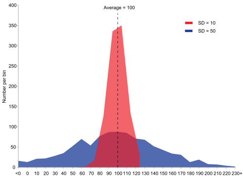
確率論と統計学において、分散はばらつきの尺度であり、つまり、一連の数値が平均値からどれだけばらついているかを示す尺度です。これは、確率変数の平均からの偏差の二乗の期待値として定義されます。標準偏差は分散の平方根です。厳密には、これは分布の2次中心モーメントであり、確率変数とそれ自身との共分散であり、多くの場合、で表されます。 $\displaystyle \sigma ^{2}}$ ⁠、 ⁠ $s²$ ⁠、 ⁠ $\operatorname {Var} (X)$ ⁠、 ⁠ $V(X)$ ⁠、または⁠ $\mathbb {V} (X)$ ⁠ .^{[ 1 ]}

分散をばらつきの尺度として用いる利点は、期待絶対偏差などの他のばらつきの尺度よりも代数的な操作が容易であることです。例えば、無相関の確率変数の和の分散は、それぞれの分散の和に等しくなります。実用的な応用において分散が不利な点は、標準偏差とは異なり、その単位が確率変数の単位と異なることです。そのため、計算が終わった後は、ばらつきの尺度として標準偏差が報告されるのが一般的です。また、多くの分布において分散が有限ではないことも不利な点です。

「分散」と呼ばれる概念には、大きく分けて2種類あります。1つは、前述のように、理論的な確率分布の一部であり、方程式で定義されます。もう1つは、観測値の集合の特性です。観測値から分散を計算する場合、それらの観測値は通常、実際のシステムから測定されます。システムのすべての観測値が存在する場合、計算された分散は母集団分散と呼ばれます。しかし、通常は一部の観測値しか得られず、そこから計算された分散は標本分散と呼ばれます。標本から計算された分散は、母集団全体の分散の推定値とみなされます。標本分散に基づいて母集団分散を推定する方法は複数あり、これについては後述します。

2種類の分散は密接に関連しています。その関係性を理解するために、理論的な確率分布を仮想的な観測値の生成器として使用できることを考えてみましょう。ある分布を用いて無限個の観測値を生成すると、その無限集合から計算された標本分散は、その分布の分散の式を用いて計算された値と一致します。分散は統計学において中心的な役割を果たしており、記述統計、統計的推論、仮説検定、適合度、モンテカルロサンプリングなど、分散を用いる概念がいくつかあります。

意味

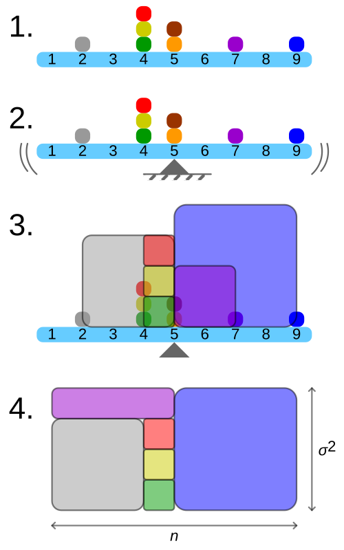
確率変数の分散 $X$ は、平均からの二乗偏差の期待値です。 $X$ ⁠、 ⁠ $\mu =\operatorname {E} [X]$ ⁠ : $\operatorname {Var} (X)=\operatorname {E} \left[(X-\mu )^{2}\right].$ この定義は、離散的、連続的、どちらでもない、または混合的なプロセスによって生成される確率変数を包含します。分散は、確率変数とそれ自身との共分散と考えることもできます。 $\operatorname {Var} (X)=\operatorname {Cov} (X,X)。$

分散は、確率分布の2番目のキュムラントにも相当し、 $X$ ⁠。分散は通常次のように指定されます。 $\operatorname {Var} (X)$ ⁠、または時々 $V(X)$ または⁠ $\mathbb {V} (X)$ ⁠、または象徴的に⁠ $\displaystyle \sigma _{X}^{2}}$ または単に $\displaystyle \sigma ^{2}}$ （「シグマ二乗」と発音します）。分散の式は次のように展開できます。 ${\begin{aligned}\operatorname {Var} (X)&=\operatorname {E} \left[{\left(X-\operatorname {E} [X]\right)}^{2}\right]\\[4pt]&=\operatorname {E} \left[X^{2}-2X\operatorname {E} [X]+\operatorname {E} [X]^{2}\right]\\[4pt]&=\operatorname {E} \left[X^{2}\right]-2\operatorname {E} [X]\operatorname {E} [X]+\operatorname {E} [X]^{2}\\[4pt]&=\operatorname {E} \left[X^{2}\right]-2\operatorname {E} [X]^{2}+\operatorname {E} [X]^{2}\\[4pt]&=\operatorname {E} \left[X^{2}\right]-\operatorname {E} [X]^{2}\end{aligned}}$

言い換えれば、の分散は $X$ はの二乗の平均に等しい $X$ 平均値の二乗を引いた値 $X$ この式は、浮動小数点演算を用いた計算には使用しないでください。式の2つの要素の大きさが似ている場合、致命的な打ち消しが発生するためです。数値的に安定した他の代替方法については、「分散を計算するためのアルゴリズム」を参照してください。

離散確率変数

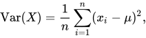
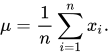
乱数発生器 $X$ 確率質量関数を持つ離散的である $x_{1}\mapsto p_{1},x_{2}\mapsto p_{2},\ldots ,x_{n}\mapsto p_{n}$ 、それから $\operatorname {Var} (X)=\sum _{i=1}^{n}p_{i}\cdot {\left(x_{i}-\mu \right)}^{2},$ どこ $\mu$ は期待値です。つまり、 $\mu =\sum _{i=1}^{n}p_{i}x_{i}.$ （このような離散的な加重分散が、合計が 1でない重みによって指定されている場合は、重みの合計で割る。）

コレクションの分散 $n$ 等確率の値は次のように表すことができます。 $\operatorname {Var} (X)={\frac {1}{n}}\sum _{i=1}^{n}(x_{i}-\mu )^{2},$ どこ $\mu$ は平均値です。つまり、 $\mu ={\frac {1}{n}}\sum _{i=1}^{n}x_{i}.$

一連の分散 $n$ 等確率の値は、平均を直接参照することなく、点同士のすべてのペアワイズ二乗距離の二乗偏差で同等に表現できます。^{[ 2 ]} $\operatorname {Var} (X)={\frac {1}{n^{2}}}\sum _{i=1}^{n}\sum _{j=1}^{n}{\frac {1}{2}}{\left(x_{i}-x_{j}\right)}^{2}={\frac {1}{n^{2}}}\sum _{i}\sum _{j>i}{\left(x_{i}-x_{j}\right)}^{2}.$

絶対連続確率変数

ランダム変数 $X$ 確率密度関数を持つ $f(x)$ ⁠、そして $F(x)$ は対応する累積分布関数であり、 ${\begin{aligned}\operatorname {Var} (X)=\sigma ^{2}&=\int _{\mathbb {R} }{\left(x-\mu \right)}^{2}f(x)\,dx\\[4pt]&=\int _{\mathbb {R} }x^{2}f(x)\,dx-2\mu \int _{\mathbb {R} }xf(x)\,dx+\mu ^{2}\int _{\mathbb {R} }f(x)\,dx\\[4pt]&=\int _{\mathbb {R} }x^{2}\,dF(x)-2\mu \int _{\mathbb {R} }x\,dF(x)+\mu ^{2}\int _{\mathbb {R} }\,dF(x)\\[4pt]&=\int _{\mathbb {R} }x^{2}\,dF(x)-2\mu \cdot \mu +\mu ^{2}\cdot 1\\[4pt]&=\int _{\mathbb {R} }x^{2}\,dF(x)-\mu ^{2},\end{aligned}}$ または同等に、 $\operatorname {Var} (X)=\int _{\mathbb {R} }x^{2}f(x)\,dx-\mu ^{2},$ どこ $\mu$ は期待値です $X$ によって与えられた $\mu =\int _{\mathbb {R} }xf(x)\,dx=\int _{\mathbb {R} }x\,dF(x).$

これらの式では、 $dx$ そして $dF(x)$ それぞれ、ルベーグ積分とルベーグ・スティルチェス積分である。

関数が $x^{2}f(x)$ 任意の有限区間でリーマン積分可能である $[a,b]\subset \mathbb {R} ,$ それから $\operatorname {Var} (X)=\int _{-\infty }^{+\infty }x^{2}f(x)\,dx-\mu ^{2},$ ここで、積分は広義リーマン積分である。

例

指数分布

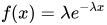
パラメータを持つ指数分布 $\lambda >0$ は連続分布であり、その確率密度関数は次のように与えられる。 $f(x)=\lambda e^{-\lambda x}$ 区間 $[0, \infty)$ 上。その平均は次のように表される。 $\operatorname {E} [X]=\int _{0}^{\infty }x\lambda e^{-\lambda x}\,dx={\frac {1}{\lambda }}.$

部分積分法を用い、既に計算済みの期待値を利用すると、次のようになります。 ${\begin{aligned}\operatorname {E} \left[X^{2}\right]&=\int _{0}^{\infty }x^{2}\lambda e^{-\lambda x}\,dx\\&={\left[-x^{2}e^{-\lambda x}\right]}_{0}^{\infty }+\int _{0}^{\infty }2xe^{-\lambda x}\,dx\\&=0+{\frac {2}{\lambda }}\operatorname {E} [X]\\&={\frac {2}{\lambda ^{2}}}.\end{aligned}}$

したがって、の分散は $X$ ⁠は次のように与えられる $\operatorname {Var} (X)=\operatorname {E} \left[X^{2}\right]-\operatorname {E} [X]^{2}={\frac {2}{\lambda ^{2}}}-\left({\frac {1}{\lambda }}\right)^{2}={\frac {1}{\lambda ^{2}}}.$

フェアダイ

公平な6面サイコロは離散確率変数としてモデル化できる。 $X$ ⁠、結果1から6までがあり、それぞれ確率は1/6です。の期待値は⁠ $X$ ⁠は $(1+2+3+4+5+6)/6=7/2.$ したがって、の分散は $X$ ⁠は ${\begin{aligned}\operatorname {Var} (X)&=\sum _{i=1}^{6}{\frac {1}{6}}\left(i-{\frac {7}{2}}\right)^{2}\\[5pt]&={\frac {1}{6}}\left((-5/2)^{2}+(-3/2)^{2}+(-1/2)^{2}+(1/2)^{2}+(3/2)^{2}+(5/2)^{2}\right)\\[5pt]&={\frac {35}{12}}\approx 2.92.\end{aligned}}$

結果の分散の一般式は、 $X$ ⁠、の⁠ $n$ ⁠面ダイスは ${\begin{aligned}\operatorname {Var} (X)&=\operatorname {E} \left(X^{2}\right)-(\operatorname {E} (X))^{2}\\[5pt]&={\frac {1}{n}}\sum _{i=1}^{n}i^{2}-\left({\frac {1}{n}}\sum _{i=1}^{n}i\right)^{2}\\[5pt]&={\frac {(n+1)(2n+1)}{6}}-\left({\frac {n+1}{2}}\right)^{2}\\[4pt]&={\frac {n^{2}-1}{12}}.\end{aligned}}$

一般的に使用される確率分布

以下の表は、一般的に用いられるいくつかの確率分布の分散を示しています。

不動産

基本特性

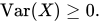
分散は非負である。なぜなら、二乗は正またはゼロだからである。 $\operatorname {Var} (X)\geq 0.$

定数の分散はゼロである。 $\operatorname {Var} (a)=0.$

逆に、確率変数の分散が0であれば、それはほぼ確実に定数である。つまり、常に同じ値をとる。 $\operatorname {Var} (X)=0\iff \exists a:P(X=a)=1.$

有限性の問題

コーシー分布のように、分布の期待値が有限でない場合、分散も有限にはなり得ません。ただし、期待値が有限であっても、分散が有限でない分布もあります。例えば、指数が 1/2であるパレート分布などが挙げられます。 $k$ 満たす $1<k\leq 2.$

分解

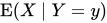
分散分解の一般式、または全分散の法則は次のとおりです。 $X$ そして $Y$ は 2 つの確率変数であり、分散は $X$ 存在するならば、 $\operatorname {Var} [X]=\operatorname {E} (\operatorname {Var} [X\mid Y])+\operatorname {Var} (\operatorname {E} [X\mid Y]).$

条件付き期待値 $\operatorname {E} (X\mid Y)$ の $X$ 与えられた $Y$ 、条件付き分散 $\operatorname {Var} (X\mid Y)$ 次のように理解できます。確率変数Yの任意の特定の値yが与えられた場合、条件付き期待値があります。 $\operatorname {E} (X\mid Y=y)$ 事象Y = yが与えられた場合、この量は特定の値yに依存します。これは関数です。 $g(y)=\operatorname {E} (X\mid Y=y)$ 同じ関数を確率変数Yで評価したものが条件付き期待値です。 $\operatorname {E} (X\mid Y)=g(Y)$ ⁠ .

特に、 $Y$ は離散確率変数であり、取りうる値をとる。 $y_{1},y_{2},y_{3}\ldots$ 対応する確率とともに $p_{1},p_{2},p_{3}\ldots ,$ すると、全分散の式において、右辺の最初の項は次のようになる。 $\operatorname {E} (\operatorname {Var} [X\mid Y])=\sum _{i}p_{i}\sigma _{i}^{2},$ どこ $\sigma _{i}^{2}=\operatorname {Var} [X\mid Y=y_{i}]$ 同様に、右辺の第２項は次のようになる。 $\operatorname {Var} (\operatorname {E} [X\mid Y])=\sum _{i}p_{i}\mu _{i}^{2}-\left(\sum _{i}p_{i}\mu _{i}\right)^{2}=\sum _{i}p_{i}\mu _{i}^{2}-\mu ^{2},$ どこで ${1}$ そして $\textstyle \mu =\sum _{i}p_{i}\mu _{i}$ したがって、総分散は次のように表されます。 $\operatorname {Var} [X]=\sum _{i}p_{i}\sigma _{i}^{2}+\left(\sum _{i}p_{i}\mu _{i}^{2}-\mu ^{2}\right).$

同様の式は分散分析にも適用され、対応する式は次のようになる。 ${\mathit {MS}}_{\text{total}}={\mathit {MS}}_{\text{between}}+{\mathit {MS}}_{\text{within}};$ ここ ${\mathit {MS}}$ は二乗平均を表します。線形回帰分析における対応する式は次のとおりです。 ${\mathit {MS}}_{\text{total}}={\mathit {MS}}_{\text{regression}}+{\mathit {MS}}_{\text{residual}}.$

これは分散の加法性からも導き出せる。なぜなら、合計（観測）スコアは予測スコアと誤差スコアの合計であり、後者2つは無相関だからである。

二乗偏差の合計 (二乗、 ${\mathit {SS}}$ ): ${\mathit {SS}}_{\text{total}}={\mathit {SS}}_{\text{between}}+{\mathit {SS}}_{\text{within}},$ ${\mathit {SS}}_{\text{total}}={\mathit {SS}}_{\text{regression}}+{\mathit {SS}}_{\text{residual}}.$

CDFからの計算

非負の確率変数の母分散は、累積分布関数Fを用いて表現できます。 $2\int _{0}^{\infty }u(1-F(u))\,du-{\left[\int _{0}^{\infty }(1-F(u))\,du\right]}^{2}.$

この式は、累積分布関数は簡単に表現できるが、密度関数は簡単に表現できないような状況で、分散を計算するために使用できます。

特性

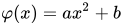
確率変数の2次モーメントは、確率変数の1次モーメント（つまり平均）付近で最小値をとる。 $\mathrm {argmin} _{m}\,\mathrm {E} \left(\left(X-m\right)^{2}\right)=\mathrm {E} (X)$ ⁠. Conversely, if a continuous function $\varphi$ satisfies $\mathrm {argmin} _{m}\,\mathrm {E} (\varphi (X-m))=\mathrm {E} (X)$ for all random variables $X$ , then it is necessarily of the form ⁠ $\varphi (x)=ax^{2}+b$ ⁠, where $a > 0$ . This also holds in the multidimensional case.^[3]

Units of measurement

Unlike the expected absolute deviation, the variance of a variable has units that are the square of the units of the variable itself. For example, a variable measured in meters will have a variance measured in meters squared. For this reason, describing data sets via their standard deviation or root mean square deviation is often preferred over using the variance. In the dice example the standard deviation is $\sqrt 2.9 \approx 1.7$ , slightly larger than the expected absolute deviation of 1.5.

The standard deviation and the expected absolute deviation can both be used as an indicator of the "spread" of a distribution. The standard deviation is more amenable to algebraic manipulation than the expected absolute deviation, and, together with variance and its generalization covariance, is used frequently in theoretical statistics; however the expected absolute deviation tends to be more robust as it is less sensitive to outliers arising from measurement anomalies or an unduly heavy-tailed distribution.

Propagation

Addition and multiplication by a constant

Variance is invariant with respect to changes in a location parameter. That is, if a constant is added to all values of the variable, the variance is unchanged: $\operatorname {Var} (X+a)=\operatorname {Var} (X).$

If all values are scaled by a constant, the variance is scaled by the square of that constant: $\operatorname {Var} (aX)=a^{2}\operatorname {Var} (X).$

The variance of a sum of two random variables is given by ${\begin{aligned}\operatorname {Var} (aX+bY)&=a^{2}\operatorname {Var} (X)+b^{2}\operatorname {Var} (Y)+2ab\,\operatorname {Cov} (X,Y)\\[1ex]\operatorname {Var} (aX-bY)&=a^{2}\operatorname {Var} (X)+b^{2}\operatorname {Var} (Y)-2ab\,\operatorname {Cov} (X,Y)\end{aligned}}$ where $\operatorname {Cov} (X,Y)$ is the covariance.

Linear combinations

In general, for the sum of $N$ random variables ⁠ $\{X_{1},\dots ,X_{N}\}$ ⁠, the variance becomes: $\operatorname {Var} \left(\sum _{i=1}^{N}X_{i}\right)=\sum _{i,j=1}^{N}\operatorname {Cov} (X_{i},X_{j})=\sum _{i=1}^{N}\operatorname {Var} (X_{i})+\sum _{i,j=1,i\neq j}^{N}\operatorname {Cov} (X_{i},X_{j}),$ see also general Bienaymé's identity.

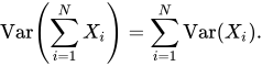
These results lead to the variance of a linear combination as: ${\begin{aligned}\operatorname {Var} \left(\sum _{i=1}^{N}a_{i}X_{i}\right)&=\sum _{i,j=1}^{N}a_{i}a_{j}\operatorname {Cov} (X_{i},X_{j})\\&=\sum _{i=1}^{N}a_{i}^{2}\operatorname {Var} (X_{i})+\sum _{i\neq j}a_{i}a_{j}\operatorname {Cov} (X_{i},X_{j})\\&=\sum _{i=1}^{N}a_{i}^{2}\operatorname {Var} (X_{i})+2\sum _{1\leq i<j\leq N}a_{i}a_{j}\operatorname {Cov} (X_{i},X_{j}).\end{aligned}}$

If the random variables $X_{1},\dots ,X_{N}$ are such that $\operatorname {Cov} (X_{i},X_{j})=0\ ,\ \forall \ (i\neq j),$ then they are said to be uncorrelated. It follows immediately from the expression given earlier that if the random variables $X_{1},\dots ,X_{N}$ are uncorrelated, then the variance of their sum is equal to the sum of their variances, or, expressed symbolically: $\operatorname {Var} \left(\sum _{i=1}^{N}X_{i}\right)=\sum _{i=1}^{N}\operatorname {Var} (X_{i}).$

Since independent random variables are always uncorrelated (see Covariance § Uncorrelatedness and independence), the equation above holds in particular when the random variables $X_{1},\dots ,X_{n}$ are independent. Thus, independence is sufficient but not necessary for the variance of the sum to equal the sum of the variances.

Matrix notation for the variance of a linear combination

Define $X$ as a column vector of $n$ random variables ⁠ $X_{1},\ldots ,X_{n}$ ⁠, and $c$ as a column vector of $n$ scalars ⁠ $c_{1},\ldots ,c_{n}$ ⁠. Therefore, $c^{\mathsf {T}}X$ is a linear combination of these random variables, where $c^{\mathsf {T}}$ denotes the transpose of ⁠ $c$ ⁠. Also let $\Sigma$ be the covariance matrix of ⁠ $X$ ⁠. The variance of $c^{\mathsf {T}}X$ is then given by:^[4] $\operatorname {Var} \left(c^{\mathsf {T}}X\right)=c^{\mathsf {T}}\Sigma c.$

This implies that the variance of the mean can be written as (with a column vector of ones) $\operatorname {Var} \left({\bar {x}}\right)=\operatorname {Var} \left({\frac {1}{n}}1'X\right)={\frac {1}{n^{2}}}1'\Sigma 1.$

Sum of variables

Sum of uncorrelated variables

One reason for the use of the variance in preference to other measures of dispersion is that the variance of the sum (or the difference) of uncorrelated random variables is the sum of their variances: $\operatorname {Var} \left(\sum _{i=1}^{n}X_{i}\right)=\sum _{i=1}^{n}\operatorname {Var} (X_{i}).$

This statement is called the Bienaymé formula^[5] and was discovered in 1853.^[6]^[7] It is often made with the stronger condition that the variables are independent, but being uncorrelated suffices. So if all the variables have the same variance $σ 2$ , then, since division by $n$ is a linear transformation, this formula immediately implies that the variance of their mean is $\operatorname {Var} \left({\overline {X}}\right)=\operatorname {Var} \left({\frac {1}{n}}\sum _{i=1}^{n}X_{i}\right)={\frac {1}{n^{2}}}\sum _{i=1}^{n}\operatorname {Var} \left(X_{i}\right)={\frac {1}{n^{2}}}n\sigma ^{2}={\frac {\sigma ^{2}}{n}}.$

That is, the variance of the mean decreases when n increases. This formula for the variance of the mean is used in the definition of the standard error of the sample mean, which is used in the central limit theorem.

To prove the initial statement, it suffices to show that $\operatorname {Var} (X+Y)=\operatorname {Var} (X)+\operatorname {Var} (Y).$

The general result then follows by induction. Starting with the definition, ${\begin{aligned}\operatorname {Var} (X+Y)&=\operatorname {E} \left[(X+Y)^{2}\right]-(\operatorname {E} [X+Y])^{2}\\[5pt]&=\operatorname {E} \left[X^{2}+2XY+Y^{2}\right]-(\operatorname {E} [X]+\operatorname {E} [Y])^{2}.\end{aligned}}$

Using the linearity of the expectation operator and the assumption of independence (or uncorrelatedness) of X and Y, this further simplifies as follows: ${\begin{aligned}\operatorname {Var} (X+Y)&=\operatorname {E} {\left[X^{2}\right]}+2\operatorname {E} [XY]+\operatorname {E} {\left[Y^{2}\right]}-\left(\operatorname {E} [X]^{2}+2\operatorname {E} [X]\operatorname {E} [Y]+\operatorname {E} [Y]^{2}\right)\\[5pt]&=\operatorname {E} \left[X^{2}\right]+\operatorname {E} \left[Y^{2}\right]-\operatorname {E} [X]^{2}-\operatorname {E} [Y]^{2}\\[5pt]&=\operatorname {Var} (X)+\operatorname {Var} (Y).\end{aligned}}$

Sum of correlated variables

Sum of correlated variables with fixed sample size

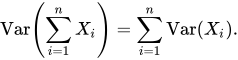
In general, the variance of the sum of $n$ variables is the sum of their covariances: $\operatorname {Var} \left(\sum _{i=1}^{n}X_{i}\right)=\sum _{i=1}^{n}\sum _{j=1}^{n}\operatorname {Cov} \left(X_{i},X_{j}\right)=\sum _{i=1}^{n}\operatorname {Var} \left(X_{i}\right)+2\sum _{1\leq i<j\leq n}\operatorname {Cov} \left(X_{i},X_{j}\right).$ $（注：2番目の等式は、Cov(X i, X i) = Var(X i)$ という事実から導かれる。）

ここ、 $\operatorname {Cov} (\cdot ,\cdot )$ は共分散であり、独立な確率変数の場合（存在する場合）はゼロになります。この式は、和の分散が、構成要素の共分散行列のすべての要素の合計に等しいことを示しています。次の式は、和の分散が共分散行列の対角要素の合計と、その上三角要素（または下三角要素）の合計の 2 倍の合計に等しいことを同等に示しています。これは、共分散行列が対称であることを強調しています。この式は、古典的テスト理論におけるクロンバックのアルファの理論で使用されています。

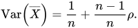
したがって、変数の分散が等しい $σ² で$ あり、異なる変数の平均相関が $ρ$ である場合、それらの平均の分散は $\operatorname {Var} \left({\overline {X}}\right)={\frac {\sigma ^{2}}{n}}+{\frac {n-1}{n}}\rho \sigma ^{2}.$

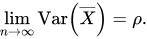
これは、平均の分散が相関の平均とともに増加することを意味します。言い換えれば、相関のある観測値を追加しても、独立した観測値を追加しても、平均の不確実性を減らす効果はそれほど高くありません。さらに、変数の分散が1である場合（例えば、標準化されている場合）、これは次のように単純化されます。 $\operatorname {Var} \left({\overline {X}}\right)={\frac {1}{n}}+{\frac {n-1}{n}}\rho .$

この式は、古典的テスト理論のスピアマン・ブラウン予測式で使用されます。平均相関が一定であるか収束する場合、nが無限大に近づくとρに収束します。 $したがって$ $、$ 相関が等しいか平均相関が収束する標準化変数の平均の分散については、次のようになります。 $\lim _{n\to \infty }\operatorname {Var} \left({\overline {X}}\right)=\rho .$

したがって、多数の標準化変数の平均の分散は、それらの平均相関にほぼ等しくなります。このことから、相関のある変数の標本平均は、独立変数の標本平均が母平均に収束するという大数の法則があるにもかかわらず、一般的には母平均に収束しないことが明らかになります。

ランダムサンプルサイズを持つ無相関変数の合計

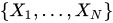
事前に、ある基準に従って許容される観測値がいくつになるか分からないままサンプルが採取される場合がある。このような場合、サンプルサイズ $Nは、その変動が$ $X$ の変動に加算される確率変数であり、^{[ 8 ]} $\operatorname {Var} \left(\sum _{i=1}^{N}X_{i}\right)=\operatorname {E} \left[N\right]\operatorname {Var} (X)+\operatorname {Var} (N)(\operatorname {E} \left[X\right])^{2}$ これは全分散の法則から導かれる。

$N$ がポアソン分布に従う場合、 $\operatorname {E} [N]=\operatorname {Var} (N)$ 推定量 $n = N$ の場合、推定量は $\textstyle \operatorname {Var} \left(\sum _{i=1}^{n}X_{i}\right)$ になる $\textstyle n{S_{x}}^{2}+n{\bar {X}}^{2}$ ⁠, giving $\textstyle \operatorname {SE} ({\bar {X}})={\sqrt {{({S_{x}}^{2}+{\bar {X}}^{2})}/{n}}}$ (see Standard error § Standard error of the sample mean).

Weighted sum of variables

The scaling property and the Bienaymé formula, along with the property of the covariance $Cov(aX, bY) = ab Cov(X, Y)$ jointly imply that $\operatorname {Var} (aX\pm bY)=a^{2}\operatorname {Var} (X)+b^{2}\operatorname {Var} (Y)\pm 2ab\,\operatorname {Cov} (X,Y).$

This implies that in a weighted sum of variables, the variable with the largest weight will have a disproportionally large weight in the variance of the total. For example, if X and Y are uncorrelated and the weight of X is two times the weight of Y, then the weight of the variance of X will be four times the weight of the variance of Y.

The expression above can be extended to a weighted sum of multiple variables: $\operatorname {Var} \left(\sum _{i}^{n}a_{i}X_{i}\right)=\sum _{i=1}^{n}a_{i}^{2}\operatorname {Var} (X_{i})+2\sum _{1\leq i}\sum _{<j\leq n}a_{i}a_{j}\operatorname {Cov} (X_{i},X_{j})$

Product of variables

Product of independent variables

If two variables X and Y are independent, the variance of their product is given by^[9] $\operatorname {Var} (XY)=[\operatorname {E} (X)]^{2}\operatorname {Var} (Y)+[\operatorname {E} (Y)]^{2}\operatorname {Var} (X)+\operatorname {Var} (X)\operatorname {Var} (Y).$

Equivalently, using the basic properties of expectation, it is given by $\operatorname {Var} (XY)=\operatorname {E} \left(X^{2}\right)\operatorname {E} \left(Y^{2}\right)-[\operatorname {E} (X)]^{2}[\operatorname {E} (Y)]^{2}.$

Product of statistically dependent variables

In general, if two variables are statistically dependent, then the variance of their product is given by:

${\begin{aligned}\operatorname {Var} (XY)={}&\operatorname {E} \left[X^{2}Y^{2}\right]-[\operatorname {E} (XY)]^{2}\\[5pt]={}&\operatorname {Cov} \left(X^{2},Y^{2}\right)+\operatorname {E} (X^{2})\operatorname {E} \left(Y^{2}\right)-[\operatorname {E} (XY)]^{2}\\[5pt]={}&\operatorname {Cov} \left(X^{2},Y^{2}\right)+\left(\operatorname {Var} (X)+[\operatorname {E} (X)]^{2}\right)\left(\operatorname {Var} (Y)+[\operatorname {E} (Y)]^{2}\right)\\[5pt]&-[\operatorname {Cov} (X,Y)+\operatorname {E} (X)\operatorname {E} (Y)]^{2}\end{aligned}}$

Arbitrary functions

The delta method uses second-order Taylor expansions to approximate the variance of a function of one or more random variables (see Taylor expansions for the moments of functions of random variables). For example, the approximate variance of a function of one variable is given by $\operatorname {Var} \left[f(X)\right]\approx \left(f'(\operatorname {E} \left[X\right])\right)^{2}\operatorname {Var} \left[X\right]$ provided that $f$ is twice differentiable and that the mean and variance of $X$ are finite.

Population variance and sample variance

Real-world observations such as the measurements of yesterday's rain throughout the day typically cannot be complete sets of all possible observations that could be made. As such, the variance calculated from the finite set will in general not match the variance that would have been calculated from the full population of possible observations. This means that one estimates the mean and variance from a limited set of observations by using an estimator equation. The estimator is a function of the sample of $n$ observations drawn without observational bias from the whole population of potential observations. In this example, the sample would be the set of actual measurements of yesterday's rainfall from available rain gauges within the geography of interest.

The simplest estimators for population mean and population variance are simply the mean and variance of the sample, the sample mean and (uncorrected) sample variance – these are consistent estimators (they converge to the value of the whole population as the number of samples increases) but can be improved. Most simply, the sample variance is computed as the sum of squared deviations about the (sample) mean, divided by $n$ as the number of samples. However, using values other than $n$ improves the estimator in various ways. Four common values for the denominator are $n$ , $n - 1$ , $n + 1$ , and $n - 1.5$ : $n$ is the simplest (the variance of the sample), $n - 1$ eliminates bias,^[10] $n + 1$ minimizes mean squared error for the normal distribution,^[11] and $n - 1.5$ mostly eliminates bias in unbiased estimation of standard deviation for the normal distribution.^[12]

Firstly, if the true population mean is unknown, then the sample variance (which uses the sample mean in place of the true mean) is a biased estimator: it underestimates the variance by a factor of $(n - 1) / n$ ; correcting this factor, resulting in the sum of squared deviations about the sample mean divided by $n - 1$ instead of $n$ , is called Bessel's correction.^[10] The resulting estimator is unbiased and is called the (corrected) sample variance or unbiased sample variance. If the mean is determined in some other way than from the same samples used to estimate the variance, then this bias does not arise, and the variance can safely be estimated as that of the samples about the (independently known) mean.

第二に、標本分散は一般的に標本分散と母集団分散の間の平均二乗誤差を最小化しません。バイアスを補正すると、多くの場合、状況が悪化します。補正された標本分散よりも優れた性能を発揮するスケールファクターを常に選択できますが、最適なスケールファクターは母集団の過剰尖度に依存し（平均二乗誤差§ 分散を参照）、バイアスを導入します。これは常に不偏推定量を縮小（ $n - 1より大きい数で割る）することによって行われ、$ 縮小推定量の簡単な例です。不偏推定量をゼロに向かって「縮小」します。正規分布の場合、 $n + 1 （$ $n - 1$ または $n$ の代わりに）で割ると、平均二乗誤差が最小化されます。^{[ 11 ]}ただし、結果として得られる推定量はバイアスがあり、バイアスのある標本変動として知られています。

母集団の分散

一般に、有限サイズの母集団の母分散は $N$ ⁠値 $x i$ は次のように与えられる ${\begin{aligned}\sigma ^{2}&={\frac {1}{N}}\sum _{i=1}^{N}{\left(x_{i}-\mu \right)}^{2}={\frac {1}{N}}\sum _{i=1}^{N}\left(x_{i}^{2}-2\mu x_{i}+\mu ^{2}\right)\\[5pt]&=\left({\frac {1}{N}}\sum _{i=1}^{N}x_{i}^{2}\right)-2\mu \left({\frac {1}{N}}\sum _{i=1}^{N}x_{i}\right)+\mu ^{2}\\[5pt]&=\operatorname {E} [x_{i}^{2}]-\mu ^{2},\end{aligned}}$ 母平均は ${\textstyle \mu =\operatorname {E} [x_{i}]={\frac {1}{N}}\sum _{i=1}^{N}x_{i}}$ そして $\textstyle \operatorname {E} [x_{i}^{2}]=\left({\frac {1}{N}}\sum _{i=1}^{N}x_{i}^{2}\right)$ ⁠、そこで ${\textstyle \operatorname {E} }$ は期待値演算子です。

母集団分散は^{[ 13 ]を用いて計算することもできる。} $\sigma ^{2}={\frac {1}{N^{2}}}\sum _{i<j}\left(x_{i}-x_{j}\right)^{2}={\frac {1}{2N^{2}}}\sum _{i,j=1}^{N}\left(x_{i}-x_{j}\right)^{2}.$

（右辺には合計に重複する項があるが、中央の辺には合計する項が重複しない。）これは、 ${\begin{aligned}&{\frac {1}{2N^{2}}}\sum _{i,j=1}^{N}{\left(x_{i}-x_{j}\right)}^{2}\\[5pt]={}&{\frac {1}{2N^{2}}}\sum _{i,j=1}^{N}\left(x_{i}^{2}-2x_{i}x_{j}+x_{j}^{2}\right)\\[5pt]={}&{\frac {1}{2N}}\sum _{j=1}^{N}\left({\frac {1}{N}}\sum _{i=1}^{N}x_{i}^{2}\right)-\left({\frac {1}{N}}\sum _{i=1}^{N}x_{i}\right)\left({\frac {1}{N}}\sum _{j=1}^{N}x_{j}\right)+{\frac {1}{2N}}\sum _{i=1}^{N}\left({\frac {1}{N}}\sum _{j=1}^{N}x_{j}^{2}\right)\\[5pt]={}&{\frac {1}{2}}\left(\sigma ^{2}+\mu ^{2}\right)-\mu ^{2}+{\frac {1}{2}}\left(\sigma ^{2}+\mu ^{2}\right)\\[5pt]={}&\sigma ^{2}.\end{aligned}}$

母集団の分散は、生成確率分布の分散と一致する。この意味で、母集団の概念は、無限母集団を持つ連続確率変数にも拡張できる。

標本分散

偏った標本分散

多くの実際的な状況では、母集団の真の分散は事前にわかっておらず、何らかの方法で計算する必要があります。非常に大きな母集団を扱う場合、母集団内のすべてのオブジェクトを数えることは不可能なので、母集団のサンプルに対して計算を実行する必要があります。 ^{[ 14 ]}これは一般にサンプル分散または経験的分散と呼ばれます。サンプル分散は、連続分布のサンプルからその分布の分散を推定するためにも適用できます。

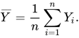
復元抽出でサンプルを採取します。 $n$ サイズの母集団からの値Y $1 、 ...、 Y n$ ⁠ $N$ ⁠、ここで $n < N$ 、このサンプルに基づいて分散を推定します。^{[ 15 ]}サンプルデータの分散を直接取ると、二乗偏差の平均が得られます。^{[ 16 ]} ${\tilde {S}}_{Y}^{2}={\frac {1}{n}}\sum _{i=1}^{n}\left(Y_{i}-{\overline {Y}}\right)^{2}=\left({\frac {1}{n}}\sum _{i=1}^{n}Y_{i}^{2}\right)-{\overline {Y}}^{2}={\frac {1}{n^{2}}}\sum _{i,j\,:\,i<j}\left(Y_{i}-Y_{j}\right)^{2}.$ （この式の導出については、§ 母集団分散の項を参照してください。）ここで、 ${\overline {Y}}$ 標本平均を表します。 ${\overline {Y}}={\frac {1}{n}}\sum _{i=1}^{n}Y_{i}.$

$Y i$ はランダムに選択されるため、 ${\overline {Y}}$ そして ${\tilde {S}}_{Y}^{2}$ は確率変数です。期待値は、サイズ ⁠ のすべての可能なサンプル ${Y i}$ のアンサンブルで平均することによって評価できます。 $n$ 人口から。 ${\tilde {S}}_{Y}^{2}$ これにより、以下が得られます。 ${\begin{aligned}\operatorname {E} [{\tilde {S}}_{Y}^{2}]&=\operatorname {E} \left[{\frac {1}{n}}\sum _{i=1}^{n}{\left(Y_{i}-{\frac {1}{n}}\sum _{j=1}^{n}Y_{j}\right)}^{2}\right]\\[5pt]&={\frac {1}{n}}\sum _{i=1}^{n}\operatorname {E} \left[Y_{i}^{2}-{\frac {2}{n}}Y_{i}\sum _{j=1}^{n}Y_{j}+{\frac {1}{n^{2}}}\sum _{j=1}^{n}Y_{j}\sum _{k=1}^{n}Y_{k}\right]\\[5pt]&={\frac {1}{n}}\sum _{i=1}^{n}\left(\operatorname {E} \left[Y_{i}^{2}\right]-{\frac {2}{n}}\left(\sum _{j\neq i}\operatorname {E} \left[Y_{i}Y_{j}\right]+\operatorname {E} \left[Y_{i}^{2}\right]\right)+{\frac {1}{n^{2}}}\sum _{j=1}^{n}\sum _{k\neq j}^{n}\operatorname {E} \left[Y_{j}Y_{k}\right]+{\frac {1}{n^{2}}}\sum _{j=1}^{n}\operatorname {E} \left[Y_{j}^{2}\right]\right)\\[5pt]&={\frac {1}{n}}\sum _{i=1}^{n}\left({\frac {n-2}{n}}\operatorname {E} \left[Y_{i}^{2}\right]-{\frac {2}{n}}\sum _{j\neq i}\operatorname {E} \left[Y_{i}Y_{j}\right]+{\frac {1}{n^{2}}}\sum _{j=1}^{n}\sum _{k\neq j}^{n}\operatorname {E} \left[Y_{j}Y_{k}\right]+{\frac {1}{n^{2}}}\sum _{j=1}^{n}\operatorname {E} \left[Y_{j}^{2}\right]\right)\\[5pt]&={\frac {1}{n}}\sum _{i=1}^{n}\left[{\frac {n-2}{n}}\left(\sigma ^{2}+\mu ^{2}\right)-{\frac {2}{n}}(n-1)\mu ^{2}+{\frac {1}{n^{2}}}n(n-1)\mu ^{2}+{\frac {1}{n}}\left(\sigma ^{2}+\mu ^{2}\right)\right]\\[5pt]&={\frac {n-1}{n}}\sigma ^{2}.\end{aligned}}$

ここ ${\textstyle \sigma ^{2}=\operatorname {E} [Y_{i}^{2}]-\mu ^{2}}$ このセクションで導出されるのは母集団分散であり、 ${\textstyle \operatorname {E} [Y_{i}Y_{j}]=\operatorname {E} [Y_{i}]\operatorname {E} [Y_{j}]=\mu ^{2}}$ 独立性により $Y_{i}$ そして $Y_{j}$ ⁠ .

したがって ${\textstyle {\tilde {S}}_{Y}^{2}}$ 母集団の分散の推定値を示す ${\textstyle \sigma ^{2}}$ それは、 ${\textstyle {\frac {n-1}{n}}}$ 期待値が ${\textstyle {\tilde {S}}_{Y}^{2}}$ 母集団分散（真の分散）よりもその係数だけ小さい。このため、 ${\textstyle {\tilde {S}}_{Y}^{2}}$ これは偏りのある標本分散と呼ばれます。

偏りのない標本分散

このバイアスを補正すると、不偏標本分散が得られ、それはと表記される。 $S^{2}$ ⁠ : $S^{2}={\frac {n}{n-1}}{\tilde {S}}_{Y}^{2}={\frac {n}{n-1}}\left[{\frac {1}{n}}\sum _{i=1}^{n}\left(Y_{i}-{\overline {Y}}\right)^{2}\right]={\frac {1}{n-1}}\sum _{i=1}^{n}\left(Y_{i}-{\overline {Y}}\right)^{2}$

どちらの推定量も、文脈からどちらのバージョンであるかが判断できる場合は、単に標本分散と呼ぶことができる。同様の証明は、連続確率分布から抽出された標本にも適用できる。

$n - 1$ という項の使用はベッセル補正と呼ばれ、標本共分散や標本標準偏差（分散の平方根）にも用いられます。平方根は凹関数であるため、分布に依存する負のバイアス（イェンセンの不等式による）が生じ、ベッセル補正を用いた補正済み標本標準偏差はバイアスを持ちます。標準偏差の不偏推定は技術的に複雑な問題ですが、正規分布の場合、 $n - 1.5$ という項を用いることでほぼ不偏推定値が得られます。

The unbiased sample variance is a U-statistic for the function $f (y 1, y 2) = (y 1 - y 2) 2 /2$ , meaning that it is obtained by averaging a 2-sample statistic over 2-element subsets of the population.

Example

For a set of numbers {10, 15, 30, 45, 57, 52, 63, 72, 81, 93, 102, 105}, if this set is the whole data population for some measurement, then variance is the population variance 932.743 as the sum of the squared deviations about the mean of this set, divided by 12 as the number of the set members. If the set is a sample from the whole population, then the unbiased sample variance can be calculated as 1017.538 that is the sum of the squared deviations about the mean of the sample, divided by 11 instead of 12. A function VAR.S in Microsoft Excel gives the unbiased sample variance while VAR.P is for population variance.

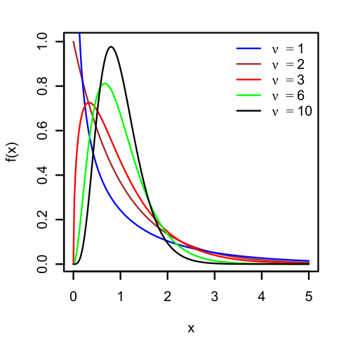
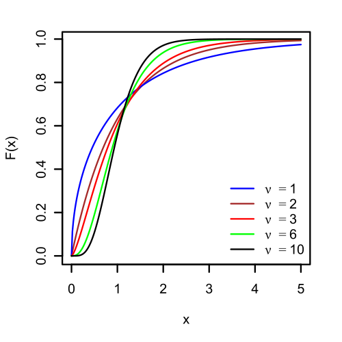
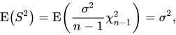
Distribution of the sample variance

Distribution and cumulative distribution of S²/σ², for various values of ν = n − 1, when the y_i are independent normally distributed.

Being a function of random variables, the sample variance is itself a random variable, and it is natural to study its distribution. In the case that Y_i are independent observations from a normal distribution, Cochran's theorem shows that the unbiased sample varianceS² follows a scaled chi-squared distribution (see also: asymptotic properties and an elementary proof):^[17] $(n-1){\frac {S^{2}}{\sigma ^{2}}}\sim \chi _{n-1}^{2},$ where $σ 2$ is the population variance. As a direct consequence, it follows that $\operatorname {E} \left(S^{2}\right)=\operatorname {E} \left({\frac {\sigma ^{2}}{n-1}}\chi _{n-1}^{2}\right)=\sigma ^{2},$ and^[18] $\operatorname {Var} \left[S^{2}\right]=\operatorname {Var} \left({\frac {\sigma ^{2}}{n-1}}\chi _{n-1}^{2}\right)={\frac {\sigma ^{4}}{{\left(n-1\right)}^{2}}}\operatorname {Var} \left(\chi _{n-1}^{2}\right)={\frac {2\sigma ^{4}}{n-1}}.$

If $Y i$ are independent and identically distributed, but not necessarily normally distributed, then^[19] $\operatorname {E} \left[S^{2}\right]=\sigma ^{2};\quad \operatorname {Var} \left[S^{2}\right]={\frac {\sigma ^{4}}{n}}\left(\kappa -1+{\frac {2}{n-1}}\right)={\frac {1}{n}}\left(\mu _{4}-{\frac {n-3}{n-1}}\sigma ^{4}\right),$ where κ is the kurtosis of the distribution and $μ 4$ is the fourth central moment.

二乗観測値に対して大数の法則の条件が満たされる場合、 $S 2は$ $σ$ $2$ の一致推定量となります。実際、推定量の分散は漸近的にゼロに近づくことがわかります。漸近的に等価な式は、Kenney と Keeping (1951:164)、Rose と Smith (2002:264)、および Weisstein (nd) で与えられています。^[²⁰^]^[²¹^]^[²²^]

サムエルソンの不平等

サムエルソンの不等式は、標本平均と（偏りのある）分散が計算されている場合、標本内の個々の観測値が取り得る値の上限を示す結果である。^{[ 23 ]}値は、以下の範囲内に収まらなければならない。 ${\bar {y}}\pm \sigma _{Y}(n-1)^{1/2}$ ⁠ .

観測値を1つ追加した場合の分散への影響

1つの新しい観測 $x_{n+1}$ セットに追加されます $n$ 平均値を持つ観測値 ${\bar {x}}_{n}$ および分散 $s_{n}^{2}$ 新しい差異 $s_{n+1}^{2}$ 再帰的な更新式を用いて表現することができる。Chan ら (1983) ^{[ 24 ]}によって提供された二乗和の恒等式に基づくと、次のようになる。

ns_{n+1}^{2}=(n-1)s_{n}^{2}+{\frac {n}{n+1}}(x_{n+1}-{\bar {x}}_{n})^{2}

この関係から、新しい観測値が分散に与える影響は、現在の平均からの距離によって決まります。 $x_{n+1}={\bar {x}}_{n}\pm s_{n}{\sqrt {\frac {n+1}{n}}}$ 、その場合、分散は変化しません。したがって、新しい観測値が平均に近い場合（ $|x_{n+1}|<{\bar {x}}_{n}+s_{n}{\sqrt {\frac {n+1}{n}}}$ ) の場合、分散は減少します。また、平均から遠ざかるほど、 $|x_{n+1}|>{\bar {x}}_{n}+s_{n}{\sqrt {\frac {n+1}{n}}}$ ) すると分散が増加します。

[証拠]

標本分散の導出

平方和の更新式を使用して（ $SS$ ):

SS_{n+1}=SS_{n}+{\frac {n}{n+1}}(x_{n+1}-{\bar {x}}_{n})^{2}

標本分散の関係を代入すると（ $SS=(n-1)s^{2}$ ):

ns_{n+1}^{2}=(n-1)s_{n}^{2}+{\frac {n}{n+1}}(x_{n+1}-{\bar {x}}_{n})^{2}

設定 $s_{n+1}^{2}=s_{n}^{2}$ :

ns_{n}^{2}=(n-1)s_{n}^{2}+{\frac {n}{n+1}}(x_{n+1}-{\bar {x}}_{n})^{2}

s_{n}^{2}={\frac {n}{n+1}}(x_{n+1}-{\bar {x}}_{n})^{2}

解決する $x_{n+1}$ 収量：

x_{n+1}={\bar {x}}_{n}\pm s_{n}{\sqrt {\frac {n+1}{n}}}

母集団分散の導出

母集団の分散については（ $\sigma ^{2}={\frac {SS}{n}}$ )更新式は次のとおりです。

(n+1)\sigma _{n+1}^{2}=n\sigma _{n}^{2}+{\frac {n}{n+1}}(x_{n+1}-\mu _{n})^{2}

設定 $\sigma _{n+1}^{2}=\sigma _{n}^{2}$ :

(n+1)\sigma _{n}^{2}=n\sigma _{n}^{2}+{\frac {n}{n+1}}(x_{n+1}-\mu _{n})^{2}

\sigma _{n}^{2}={\frac {n}{n+1}}(x_{n+1}-\mu _{n})^{2}

解決する $x_{n+1}$ 収量：

x_{n+1}=\mu _{n}\pm \sigma _{n}{\sqrt {\frac {n+1}{n}}}

調和平均と算術平均との関係

^正の^実数のサンプル ${$ ^y $i$ $}$ に対して $、$ $\sigma _{y}^{2}\leq 2y_{\max }(A-H),$ ここで、 $y max$ はサンプルの最大値であり、 $A$ は算術平均です。 $H$ はサンプルの調和平均であり、 $\sigma _{y}^{2}$ これは標本の（偏りのある）分散です。

この境界は改善され、分散は以下によって制限されることが知られています。 ${\begin{aligned}\sigma _{y}^{2}&\leq {\frac {y_{\max }(A-H)(y_{\max }-A)}{y_{\max }-H}},\\[1ex]\sigma _{y}^{2}&\geq {\frac {y_{\min }(A-H)(A-y_{\min })}{H-y_{\min }}},\end{aligned}}$ ここで、 $y min$ はサンプルの最小値である。^{[ 26 ]}

分散の等質性検定

標本が正規分布に従う場合、分散の等質性を検定するF検定とカイ二乗検定は適切である。正規分布に従わない場合、2つ以上の分散の等質性を検定することはより困難になる。

ノンパラメトリック検定がいくつか提案されている。これには、バートン・デイビッド・アンサリ・フロイント・シーゲル・テューキー検定、カポン検定、ムード検定、クロッツ検定、スカトメ検定などがある。スカトメ検定は2つの分散に適用され、両方のメジアンが既知でゼロに等しい必要がある。ムード検定、クロッツ検定、カポン検定、バートン・デイビッド・アンサリ・フロイント・シーゲル・テューキー検定も2つの分散に適用され、メジアンが未知であってもよいが、2つのメジアンが等しい必要がある。

レーマン検定は、2つの分散を比較するパラメトリック検定です。この検定にはいくつかのバリエーションが知られています。分散の等質性を検定する他の方法としては、ボックス検定、ボックス・アンダーソン検定、モーゼス検定などがあります。

ブートストラップ法やジャックナイフ法などのリサンプリング法は、分散の等質性を検定するために使用できる。

慣性モーメント

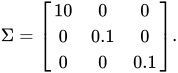
確率分布の分散は、古典力学における、重心周りの回転に関する、線に沿った対応する質量分布の慣性モーメントに類似している。 ^[²⁷^]この類似性から、分散のようなものは確率分布のモーメント と呼ばれる。^[²⁷^]共分散行列は、多変量分布の慣性モーメントテンソルと関連している。共分散行列を持つn個の点のクラウドの慣性モーメントは、 $\Sigma$ は $I=n\left(\mathbf {1} _{3\times 3}\operatorname {tr} (\Sigma )-\Sigma \right).$

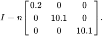
物理学と統計学における慣性モーメントの違いは、直線上に集まった点の場合に明らかです。多くの点がx軸の近くにあり、x軸に沿って分布していると仮定します。共分散行列は次のようになります。 $\Sigma ={\begin{bmatrix}10&0&0\\0&0.1&0\\0&0&0.1\end{bmatrix}}.$

つまり、 x方向の変動が最も大きい。物理学者はこれをx軸周りのモーメントが小さいとみなすので、慣性モーメントテンソルは $I=n{\begin{bmatrix}0.2&0&0\\0&10.1&0\\0&0&10.1\end{bmatrix}}.$

半分散

半分散は分散と同じ方法で計算されますが、計算には平均値より低い観測値のみが含まれます。 ${\text{Semivariance}}={\frac {1}{n}}\sum _{i:x_{i}<\mu }{\left(x_{i}-\mu \right)}^{2}$ また、さまざまな応用分野において、特定の尺度として説明されています。歪んだ分布の場合、半分散は分散では得られない追加情報を提供できます。^{[ 28 ]}

半変性に関連する不等式については、チェビシェフの不等式 § 半変性を参照してください。

語源

分散という用語は、ロナルド・フィッシャーが1918年の論文「メンデル遺伝の仮定に基づく親族間の相関」で初めて導入した。^{[ 29 ]}

入手可能な膨大な統計データは、人間の測定値の平均値からの偏差が正規誤差法則に非常に近いことを示し、したがって、変動性は平均二乗誤差の平方根に対応する標準偏差によって一様に測定できることを示しています。均一な母集団分布に標準偏差を持つ2つの独立した変動原因が存在する場合、 $\sigma _{1}$ そして $\sigma _{2}$ 両方の原因が同時に作用する場合、分布の標準偏差は ${\sqrt {\sigma _{1}^{2}+\sigma _{2}^{2}}}$ したがって、変動の原因を分析する際には、変動の尺度として標準偏差の二乗を用いることが望ましい。この量を分散と呼ぶことにする。

一般化

複素変数の場合

もし $x$ は、の値をとるようなスカラー複素数値確率変数です。 $\mathbb {C}$ ⁠、その分散は⁠ $\operatorname {E} \left[(x-\mu )(x-\mu )^{*}\right]$ ⁠、そこで $x^{*}$ はの複素共役です $x$ この分散は実数スカラーです。

ベクトル値確率変数の場合

行列として

もし $X$ は、値の範囲がであるベクトル値確率変数です。 $\mathbb {R} ^{n},$ 列ベクトルとして考えると、分散の自然な一般化は次のようになる。 $\operatorname {E} \left[(X-\mu ){(X-\mu )}^{\mathsf {T}}\right],$ どこ $\mu =\operatorname {E} (X)$ そして $X^{\mathsf {T}}$ はの転置です $X$ ⁠、そして行ベクトルです。結果として得られるのは正の半正定値正方行列で、一般に分散共分散行列（または単に共分散行列）と呼ばれます。

もし $X$ は、値の範囲がであるベクトル値かつ複素数値の確率変数です。 $\mathbb {C} ^{n}$ ⁠、すると共分散行列は⁠ $\operatorname {E} \left[(X-\mu ){(X-\mu )}^{\dagger }\right]$ ⁠、そこで $X^{\dagger }$ はの共役転置です $X$ この行列は正半定値かつ正方行列です。

スカラーとして

ベクトル値確率変数の分散に関する別の一般化 $X,$ 行列ではなくスカラー値となるのは、一般化分散である。 $\det(C)$ 共分散行列の行列式。一般化分散は、点の平均値を中心とした多次元散布と関連していることが示される。^{[ 30 ]}

スカラー分散の式を考慮すると、別の一般化が得られる。 $\operatorname {Var} (X)=\operatorname {E} \left[(X-\mu )^{2}\right],$ そして再解釈する $(X-\mu )^{2}$ 確率変数とその平均値との間のユークリッド距離の二乗、または単にベクトルのスカラー積として $X-\mu$ それ自体と。その結果、 $\operatorname {E} \left[(X-\mu )^{\mathsf {T}}(X-\mu )\right]=\operatorname {tr} (C),$ これは共分散行列のトレースです。

参考文献

↑ワッサーマン、ラリー（2005）。統計学のすべて：統計的推論の簡潔なコース。シュプリンガー統計学テキスト。51 ページ。ISBN 978-1-4419-2322-6。
↑ Yuli Zhang; Huaiyu Wu; Lei Cheng (2012年6月).分散と共分散に関するいくつかの新しい変形式. 第4回モデリング、識別、制御に関する国際会議(ICMIC2012)論文集. pp. 987–992 .
↑ Kagan, A.; Shepp, LA (1998). "Why the variance?". Statistics & Probability Letters . 38 (4): 329– 333. doi : 10.1016/S0167-7152(98)00041-8 .
↑ジョンソン、リチャード；ウィチャーン、ディーン（2001）。応用多変量統計解析。プレンティスホール。76ページ。ISBN 0-13-187715-1。
↑ Loève, M. (1977) 「確率論」、大学院数学テキスト、第45巻、第4版、Springer-Verlag、p. 12。
↑ビエネイメ、I.-J. (1853) "Considérations à l'appui de la découverte de Laplace sur la loi de probabilité dans la methode des moindres carrés"、 Comptes rendus de l'Académie des Sciences Paris、37、p. 309–317;デジタルコピーが利用可能Wayback Machineに2018年6月23日にアーカイブされました
↑ビエネイメ、I.-J. (1867) "Considérations à l'appui de la découverte de Laplace sur la loi de probabilité dans la methode des moindres carrés"、 Journal de Mathématiques Pures et Appliquées、Série 2、Tome 12、p. 158–167;デジタルコピーが利用可能
↑ Cornell, JR、および Benjamin, CA、『土木技術者のための確率、統計、および意思決定』、McGraw-Hill、ニューヨーク、1970 年、178-9 ページ。
↑ Goodman, Leo A. (1960 年 12 月). 「製品の正確な分散について」. Journal of the American Statistical Association . 55 (292): 708–713 . doi : 10.2307/2281592 . JSTOR 2281592 .
1 2ライヒマン、WJ (1961)。「付録 8」。統計の利用と濫用（ペリカン版、1964～1970年再版）。ロンドン：メシュエン。
1 2 Kourouklis, Stavros (2012). "平均二乗誤差を最小化する分散の新しい推定量" .The American Statistician . 66 (4): 234–236 . doi : 10.1080/00031305.2012.735209 . ISSN 0003-1305 . JSTOR 23339501 .
↑ Brugger, RM (1969). "標準偏差の不偏推定に関する注記". The American Statistician . 23 (4): 32. doi : 10.1080/00031305.1969.10481865 .
↑ Yuli Zhang; Huaiyu Wu; Lei Cheng (2012年6月).分散と共分散に関するいくつかの新しい変形式. 第4回モデリング、識別、制御に関する国際会議(ICMIC2012)論文集. pp. 987–992 .
↑ Navidi, William (2006). Statistics for Engineers and Scientists . McGraw-Hill. p. 14.
↑ Montgomery, DC および Runger, GC (1994)『エンジニアのための応用統計学と確率論』、201 ページ。John Wiley & Sons、ニューヨーク
↑ Yuli Zhang; Huaiyu Wu; Lei Cheng (2012年6月).分散と共分散に関するいくつかの新しい変形式. 第4回モデリング、識別、制御に関する国際会議(ICMIC2012)論文集. pp. 987–992 .
↑ Knight, K. (2000). Mathematical Statistics . New York: Chapman and Hall. 命題 2.11.
↑ Casella, George ; Berger, Roger L. (2002).統計的推論（第2版）. 例7.3.3、p. 331. ISBN 0-534-24312-6。
↑ Mood, AM、Graybill, FA、Boes, DC (1974)『統計理論入門』第3版、McGraw-Hill、ニューヨーク、p. 229
↑ Kenney, John F.; Keeping, ES (1951).統計学の数学。パート2 (PDF) (第2版)。プリンストン、ニュージャージー州: D. Van Nostrand Company, Inc. 2018年11月17日にオリジナル(PDF)からアーカイブ- KrishiKosh 経由。
↑ Rose, Colin; Smith, Murray D. (2002). " Mathematicaによる数理統計学". Springer-Verlag、ニューヨーク。
↑ Weisstein, Eric W. 「サンプル分散分布」。MathWorld Wolfram。
↑ Samuelson, Paul (1968). "How Deviant Can You Be?". Journal of the American Statistical Association . 63 (324): 1522– 1525. doi : 10.1080/01621459.1968.10480944 . JSTOR 2285901 .
↑ Chan, Tony F.; Golub, Gene H.; LeVeque, Randall J. (1983). "標本分散を計算するためのアルゴリズム: 分析と推奨事項" . The American Statistician . 37 (3): 242– 247. doi : 10.2307/2683386 .式1.3(b 1ページ目)
↑ Mercer, A. McD. (2000). "一般的な方法を用いた A–G、A–H、G–H、および Ky Fan 型の不等式の族の境界" . J. Math. Anal. Appl . 243 (1): 163– 173. doi : 10.1006/jmaa.1999.6688 .
↑ Sharma, R. (2008). "算術平均、調和平均、分散に関するその他の不等式". Journal of Mathematical Inequalities . 2 (1): 109– 114. CiteSeerX 10.1.1.551.9397 . doi : 10.7153/jmi-02-11 .
1 2 Magnello, M. Eileen. 「カール・ピアソンと現代統計学の起源：弾性論者が統計学者になる」。ラザフォード・ジャーナル。
↑ Fama, Eugene F.; French, Kenneth R. (2010-04-21). "Q&A: 半分散: より良いリスク尺度か? . Fama/French Forum .
↑ロナルド・フィッシャー（1918）メンデル遺伝の仮定に基づく親族間の相関関係
↑ Kocherlakota, S.; Kocherlakota, K. (2004). "Generalized Variance".Encyclopedia of Statistical Sciences . Wiley Online Library. doi : 10.1002/0471667196.ess0869 . ISBN 0-471-66719-6。

[1] ワッサーマン、ラリー（2005）。統計学のすべて：統計的推論の簡潔なコース。シュプリンガー統計学テキスト。51 ページ。ISBN 978-1-4419-2322-6。

[2] Yuli Zhang; Huaiyu Wu; Lei Cheng (2012年6月).分散と共分散に関するいくつかの新しい変形式. 第4回モデリング、識別、制御に関する国際会議(ICMIC2012)論文集. pp. 987–992 .

[3] Kagan, A.; Shepp, LA (1998). "Why the variance?". Statistics & Probability Letters . 38 (4): 329– 333. doi : 10.1016/S0167-7152(98)00041-8 .

[4] ジョンソン、リチャード；ウィチャーン、ディーン（2001）。応用多変量統計解析。プレンティスホール。76ページ。ISBN 0-13-187715-1。

[5] Loève, M. (1977) 「確率論」、大学院数学テキスト、第45巻、第4版、Springer-Verlag、p. 12。

[6] ビエネイメ、I.-J. (1853) "Considérations à l'appui de la découverte de Laplace sur la loi de probabilité dans la methode des moindres carrés"、 Comptes rendus de l'Académie des Sciences Paris、37、p. 309–317;デジタルコピーが利用可能Wayback Machineに2018年6月23日にアーカイブされました

[7] ビエネイメ、I.-J. (1867) "Considérations à l'appui de la découverte de Laplace sur la loi de probabilité dans la methode des moindres carrés"、 Journal de Mathématiques Pures et Appliquées、Série 2、Tome 12、p. 158–167;デジタルコピーが利用可能

[8] Cornell, JR、および Benjamin, CA、『土木技術者のための確率、統計、および意思決定』、McGraw-Hill、ニューヨーク、1970 年、178-9 ページ。

[9] Goodman, Leo A. (1960 年 12 月). 「製品の正確な分散について」. Journal of the American Statistical Association . 55 (292): 708–713 . doi : 10.2307/2281592 . JSTOR 2281592 .

[bessel-10] 1 2ライヒマン、WJ (1961)。「付録 8」。統計の利用と濫用（ペリカン版、1964～1970年再版）。ロンドン：メシュエン。

[Kourouklis-11] 1 2 Kourouklis, Stavros (2012). "平均二乗誤差を最小化する分散の新しい推定量" .The American Statistician . 66 (4): 234–236 . doi : 10.1080/00031305.2012.735209 . ISSN 0003-1305 . JSTOR 23339501 .

[12] Brugger, RM (1969). "標準偏差の不偏推定に関する注記". The American Statistician . 23 (4): 32. doi : 10.1080/00031305.1969.10481865 .

[13] Yuli Zhang; Huaiyu Wu; Lei Cheng (2012年6月).分散と共分散に関するいくつかの新しい変形式. 第4回モデリング、識別、制御に関する国際会議(ICMIC2012)論文集. pp. 987–992 .

[14] Navidi, William (2006). Statistics for Engineers and Scientists . McGraw-Hill. p. 14.

[15] Montgomery, DC および Runger, GC (1994)『エンジニアのための応用統計学と確率論』、201 ページ。John Wiley & Sons、ニューヨーク

[16] Yuli Zhang; Huaiyu Wu; Lei Cheng (2012年6月).分散と共分散に関するいくつかの新しい変形式. 第4回モデリング、識別、制御に関する国際会議(ICMIC2012)論文集. pp. 987–992 .

[17] Knight, K. (2000). Mathematical Statistics . New York: Chapman and Hall. 命題 2.11.

[18] Casella, George ; Berger, Roger L. (2002).統計的推論（第2版）. 例7.3.3、p. 331. ISBN 0-534-24312-6。

[19] Mood, AM、Graybill, FA、Boes, DC (1974)『統計理論入門』第3版、McGraw-Hill、ニューヨーク、p. 229

[20] Kenney, John F.; Keeping, ES (1951).統計学の数学。パート2 (PDF) (第2版)。プリンストン、ニュージャージー州: D. Van Nostrand Company, Inc. 2018年11月17日にオリジナル(PDF)からアーカイブ- KrishiKosh 経由。

[21] Rose, Colin; Smith, Murray D. (2002). " Mathematicaによる数理統計学". Springer-Verlag、ニューヨーク。

[22] Weisstein, Eric W. 「サンプル分散分布」。MathWorld Wolfram。

[23] Samuelson, Paul (1968). "How Deviant Can You Be?". Journal of the American Statistical Association . 63 (324): 1522– 1525. doi : 10.1080/01621459.1968.10480944 . JSTOR 2285901 .

[24] Chan, Tony F.; Golub, Gene H.; LeVeque, Randall J. (1983). "標本分散を計算するためのアルゴリズム: 分析と推奨事項" . The American Statistician . 37 (3): 242– 247. doi : 10.2307/2683386 .式1.3(b 1ページ目)

[25] Mercer, A. McD. (2000). "一般的な方法を用いた A–G、A–H、G–H、および Ky Fan 型の不等式の族の境界" . J. Math. Anal. Appl . 243 (1): 163– 173. doi : 10.1006/jmaa.1999.6688 .

[Sharma2008-26] Sharma, R. (2008). "算術平均、調和平均、分散に関するその他の不等式". Journal of Mathematical Inequalities . 2 (1): 109– 114. CiteSeerX 10.1.1.551.9397 . doi : 10.7153/jmi-02-11 .

[pearson-27] 1 2 Magnello, M. Eileen. 「カール・ピアソンと現代統計学の起源：弾性論者が統計学者になる」。ラザフォード・ジャーナル。

[28] Fama, Eugene F.; French, Kenneth R. (2010-04-21). "Q&A: 半分散: より良いリスク尺度か? . Fama/French Forum .

[29] ロナルド・フィッシャー（1918）メンデル遺伝の仮定に基づく親族間の相関関係

[30] Kocherlakota, S.; Kocherlakota, K. (2004). "Generalized Variance".Encyclopedia of Statistical Sciences . Wiley Online Library. doi : 10.1002/0471667196.ess0869 . ISBN 0-471-66719-6。

[ 1 ]

[ 2 ]

[3]

[4]

[5]

[6]

[7]

[ 8 ]

[9]

[10]

[11]

[12]

[ 13 ]を用いて計算することもできる。

[ 14 ]

[ 15 ]

[ 16 ]

[17]

[18]

[19]

[

[

[

[ 23 ]

[ 24 ]

正の

[ 26 ]

[

[ 28 ]

[ 29 ]

[ 30 ]

意味