ベクトル束の特性類
In mathematics , in particular in algebraic topology , differential geometry and algebraic geometry , the Chern classes are characteristic classes associated with complex vector bundles . They have since become fundamental concepts in many branches of mathematics and physics, such as string theory , Chern–Simons theory , knot theory , Gromov–Witten invariants .
Chern classes were introduced by Shiing-Shen Chern (1946).
Geometric approach
Basic idea and motivation
Chern classes are characteristic classes . They are topological invariants associated with vector bundles on a smooth manifold. The question of whether two ostensibly different vector bundles are the same can be quite hard to answer. The Chern classes provide a simple test: if the Chern classes of a pair of vector bundles do not agree, then the vector bundles are different. The converse, however, is not true.
In topology, differential geometry, and algebraic geometry, it is often important to count how many linearly independent sections a vector bundle has. The Chern classes offer some information about this through, for instance, the Riemann–Roch theorem and the Atiyah–Singer index theorem .
Chern classes are also feasible to calculate in practice. In differential geometry (and some types of algebraic geometry), the Chern classes can be expressed as polynomials in the coefficients of the curvature form .
Construction
There are various ways of approaching the subject, each of which focuses on a slightly different flavor of Chern class.
The original approach to Chern classes was via algebraic topology: the Chern classes arise via homotopy theory which provides a mapping associated with a vector bundle to a classifying space (an infinite Grassmannian in this case). For any complex vector bundle V over a manifold M , there exists a map f from M to the classifying space such that the bundle V is equal to the pullback, by f , of a universal bundle over the classifying space, and the Chern classes of V can therefore be defined as the pullback of the Chern classes of the universal bundle. In turn, these universal Chern classes can be explicitly written down in terms of Schubert cycles .
M から 分類空間への任意の 2 つの写像 f 、 gについて、その引き戻しが同じバンドル V である場合、写像はホモトピックでなければならないことが示されます。したがって、 f または gのいずれかによる任意の普遍チャーン類の M のコホモロジー類への引き戻しは、同じ類でなければなりません。これは、 V のチャーン類 が明確に定義されていることを示しています。
チャーンのアプローチは、この記事で主に説明されている曲率アプローチを介して微分幾何学を使用しました。彼は、以前の定義が実際には彼の定義と同等であることを示しました。結果として得られた理論は、 チャーン-ワイル理論 として知られています。
アレクサンダー・グロタンディーク のアプローチもあり、 公理的には線束の場合のみを定義する必要があることを示しています。
チャーン類は代数幾何学 で自然に生じます 。代数幾何学における一般化されたチャーン類は、任意の非特異多様体上のベクトル束(より正確には、 局所自由層 )に対して定義できます。代数幾何学的チャーン類では、基礎となる体が特別な特性を持つことは要求されません。特に、ベクトル束は必ずしも複素数である必要はありません。
特定のパラダイムに関係なく、チャーン類の直感的な意味は、 ベクトル束の セクションの「必要なゼロ」に関係しています。たとえば、毛玉を平らに梳かすことはできないという定理 ( 毛玉定理) などです。これは厳密に言えば 実数 ベクトル束に関する質問ですが (球の「毛」は実際には実数線のコピーです)、毛が複素数である場合 (以下の複素毛玉定理の例を参照)、または他の多くのフィールド上の 1 次元射影空間の場合の一般化があります。
詳しい議論については、 Chern-Simons 理論 を参照してください 。
直線束のチャーン類 ( X を CW 複体 の ホモトピー型 を持つ位相空間とします 。)
Vが 直線束 の とき、重要な特殊なケースが発生します。その場合、唯一の非自明なチャーン類は、 X の2番目のコホモロジー群の要素である最初のチャーン類です 。これは最上位のチャーン類であるため、 束の
オイラー類に等しくなります。
最初のチャーン類は、 位相的に言えば、複素直線束を分類するための 完全な不変量であることが判明した。つまり、 X 上の直線束の同型類 と の元の間には 一対一の関係 があり、直線束に最初のチャーン類が関連付けられる。さらに、この一対一の関係は群準同型 (したがって同型) である。
複素直線束の
テンソル 積は、 2 番目のコホモロジー群の加算に対応する。 [1] [2]
H
2
( バツ ;
ず
)
{\displaystyle H^{2}(X;\mathbb {Z} )}
c
1
(
L
⊗
L
′
)
=
c
1
(
L
)
+
c
1
(
L
′
)
;
{\displaystyle c_{1}(L\otimes L')=c_{1}(L)+c_{1}(L');}
代数幾何学において、複素直線束(の同型類)を第一チャーン類で分類することは、正則直線束(の同型類)を 因子の 線型同値 類 で 分類することの大まかな近似である 。
1 より大きい次元の複素ベクトル束の場合、チャーン類は完全な不変量ではありません。
建設
チャーン・ワイル理論による 滑らかな多様体 M 上の 複素階数 n の複素 エルミート ベクトル束 V が与えられた場合、 V の 各チャーン類( チャーン形式 とも呼ばれる)の代表は、 V の 曲率形式 の 特性多項式 の係数として与えられます 。
c
k
(
V
)
{\displaystyle c_{k}(V)}
Ω
{\displaystyle \Omega }
det
(
i
t
Ω
2
π
+
I
)
=
∑
k
c
k
(
V
)
t
k
{\displaystyle \det \left({\frac {it\Omega }{2\pi }}+I\right)=\sum _{k}c_{k}(V)t^{k}}
行列式は、 M 上の偶複素微分形式の可換代数に係数を 持つ t の多項式を要素とする行列の環上にあります 。 V の 曲率形式は
、 ω が 接続形式 、 d が 外導関数 である として定義されるか
、または ω が V の ゲージ群 の ゲージ場 である同じ式を介して定義されます 。スカラー t は、ここでは行列式から和 を生成する ための 不定値 としてのみ使用され 、 I は n × n 単位行列 を表します 。
n
×
n
{\displaystyle n\times n}
Ω
{\displaystyle \Omega }
Ω
=
d
ω
+
1
2
[
ω
,
ω
]
{\displaystyle \Omega =d\omega +{\frac {1}{2}}[\omega ,\omega ]}
与えられた式が チャーン類の 代表であると言うことは、ここでの「類」が 正確な微分形式 の追加 までを 意味することを示しています。つまり、チャーン類は、 ド・ラーム・コホモロジー の意味で コホモロジー類です。チャーン形式のコホモロジー類は、 V の接続の選択に依存しないことがわかります 。
行列の恒等式から が成り立つ場合、 となります 。 にマクローリン級数を適用すると 、 チャーン 形式について次の式が得られます。
t
r
(
ln
(
X
)
)
=
ln
(
det
(
X
)
)
{\displaystyle \mathrm {tr} (\ln(X))=\ln(\det(X))}
det
(
X
)
=
exp
(
t
r
(
ln
(
X
)
)
)
{\displaystyle \det(X)=\exp(\mathrm {tr} (\ln(X)))}
ln
(
X
+
I
)
{\displaystyle \ln(X+I)}
∑
k
c
k
(
V
)
t
k
=
[
I
+
i
t
r
(
Ω
)
2
π
t
+
t
r
(
Ω
2
)
−
t
r
(
Ω
)
2
8
π
2
t
2
+
i
−
2
t
r
(
Ω
3
)
+
3
t
r
(
Ω
2
)
t
r
(
Ω
)
−
t
r
(
Ω
)
3
48
π
3
t
3
+
⋯
]
.
{\displaystyle \sum _{k}c_{k}(V)t^{k}=\left[I+i{\frac {\mathrm {tr} (\Omega )}{2\pi }}t+{\frac {\mathrm {tr} (\Omega ^{2})-\mathrm {tr} (\Omega )^{2}}{8\pi ^{2}}}t^{2}+i{\frac {-2\mathrm {tr} (\Omega ^{3})+3\mathrm {tr} (\Omega ^{2})\mathrm {tr} (\Omega )-\mathrm {tr} (\Omega )^{3}}{48\pi ^{3}}}t^{3}+\cdots \right].}
オイラークラス経由 チャーン類はオイラー類の観点から定義することができます。これはミルナーとスタシェフの著書におけるアプローチであり、 ベクトル束の方向 の役割を強調しています。
基本的な観察は、 複素ベクトル束は 、最終的には連結であるため、標準的な方向性を持つということです 。したがって、バンドルの最上位のチャーン類をオイラー類 (基礎となる実ベクトル束のオイラー類) として定義し、下位のチャーン類を帰納的に処理します。
GL
n
(
C
)
{\displaystyle \operatorname {GL} _{n}(\mathbb {C} )}
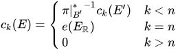
正確な構築は次の通り。アイデアは、基底変換を行ってランクが 1 少ないバンドルを得るというものである。 を パラコンパクト空間 B 上の複素ベクトルバンドルとする 。 Bが E にゼロセクションとして 埋め込まれていると考え、 とし 、新しいベクトルバンドルを定義する。
各ファイバーは、 E の
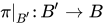
ファイバー Fを F 内の非ゼロベクトル v が張る直線で割った商となる ( B′ の点は、 E の ファイバー Fと F 上の非ゼロベクトルによって指定される ) [3]。 すると、は E のランクより 1 低いランクを持つ 。 ファイバーバンドルの Gysin シーケンス から、
は の同型である
ことが分かる 。
π
:
E
→
B
{\displaystyle \pi \colon E\to B}
B
′
=
E
∖
B
{\displaystyle B'=E\setminus B}
E
′
→
B
′
{\displaystyle E'\to B'}
E
′
{\displaystyle E'}
π
|
B
′
:
B
′
→
B
{\displaystyle \pi |_{B'}\colon B'\to B}
⋯
→
H
k
(
B
;
Z
)
→
π
|
B
′
∗
H
k
(
B
′
;
Z
)
→
⋯
,
{\displaystyle \cdots \to \operatorname {H} ^{k}(B;\mathbb {Z} ){\overset {\pi |_{B'}^{*}}{\to }}\operatorname {H} ^{k}(B';\mathbb {Z} )\to \cdots ,}
π
|
B
′
∗
{\displaystyle \pi |_{B'}^{*}}
k
<
2
n
−
1
{\displaystyle k<2n-1}
c
k
(
E
)
=
{
π
|
B
′
∗
−
1
c
k
(
E
′
)
k
<
n
e
(
E
R
)
k
=
n
0
k
>
n
{\displaystyle c_{k}(E)={\begin{cases}{\pi |_{B'}^{*}}^{-1}c_{k}(E')&k<n\\e(E_{\mathbb {R} })&k=n\\0&k>n\end{cases}}}
次に、この定義に対してチャーン類の公理が満たされているかどうかを確認するために、いくらかの作業が必要になります。
トム同型性 も参照してください 。
例
リーマン球面の複素接束 をリーマン球面 : 1 次元 複素射影空間 とします 。z はリーマン球面の正則局所座標であるとします 。 各点で の形を持つ複素接ベクトルの束を とします。 ここ で a は 複素数 です 。 毛 球定理 の複素バージョンを証明します 。V に はどこでもゼロでない断面はありません。
C
P
1
{\displaystyle \mathbb {CP} ^{1}}
V
=
T
C
P
1
{\displaystyle V=T\mathbb {CP} ^{1}}
a
∂
/
∂
z
{\displaystyle a\partial /\partial z}
このためには、次の事実が必要である:自明バンドルの最初のチャーン類はゼロである、すなわち、
c
1
(
C
P
1
×
C
)
=
0.
{\displaystyle c_{1}(\mathbb {CP} ^{1}\times \mathbb {C} )=0.}
これは、自明な束が常に平坦な接続を持つという事実によって証明される。そこで、
c
1
(
V
)
≠
0.
{\displaystyle c_{1}(V)\not =0.}
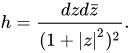
ケーラー計量 を考える
h
=
d
z
d
z
¯
(
1
+
|
z
|
2
)
2
.
{\displaystyle h={\frac {dzd{\bar {z}}}{(1+|z|^{2})^{2}}}.}
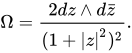
曲率2形式は次のように与えられることが容易にわかる。
Ω
=
2
d
z
∧
d
z
¯
(
1
+
|
z
|
2
)
2
.
{\displaystyle \Omega ={\frac {2dz\wedge d{\bar {z}}}{(1+|z|^{2})^{2}}}.}
さらに、第一チャーン類の定義により
c
1
=
[
i
2
π
tr
Ω
]
.
{\displaystyle c_{1}=\left[{\frac {i}{2\pi }}\operatorname {tr} \Omega \right].}
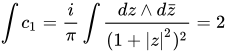
このコホモロジー類がゼロでないことを示さなければなりません。極座標
に切り替えた後 、リーマン球面上で積分を計算すれば十分です
。 ストークスの定理 により 、 正確な形式は 0 に積分されるため、コホモロジー類はゼロではありません。
∫
c
1
=
i
π
∫
d
z
∧
d
z
¯
(
1
+
|
z
|
2
)
2
=
2
{\displaystyle \int c_{1}={\frac {i}{\pi }}\int {\frac {dz\wedge d{\bar {z}}}{(1+|z|^{2})^{2}}}=2}
これは、 が自明なベクトル束ではないことを証明します。
T
C
P
1
{\displaystyle T\mathbb {CP} ^{1}}
複素射影空間 層/束の正確な列が存在する: [4]
ここで、 は構造層(すなわち、自明な直線束)、 は セールのねじれ層 (すなわち、 超平面束 )、最後の非ゼロ項は 接層 /束である。
0
→
O
C
P
n
→
O
C
P
n
(
1
)
⊕
(
n
+
1
)
→
T
C
P
n
→
0
{\displaystyle 0\to {\mathcal {O}}_{\mathbb {CP} ^{n}}\to {\mathcal {O}}_{\mathbb {CP} ^{n}}(1)^{\oplus (n+1)}\to T\mathbb {CP} ^{n}\to 0}
O
C
P
n
{\displaystyle {\mathcal {O}}_{\mathbb {CP} ^{n}}}
O
C
P
n
(
1
)
{\displaystyle {\mathcal {O}}_{\mathbb {CP} ^{n}}(1)}
上記のシーケンスを取得するには 2 つの方法があります。
[5] を の座標とし、 を 正 準射影とし、 とすると、次式が 成り立ち ます。
z
0
,
…
,
z
n
{\displaystyle z_{0},\ldots ,z_{n}}
C
n
+
1
,
{\displaystyle \mathbb {C} ^{n+1},}
π
:
C
n
+
1
∖
{
0
}
→
C
P
n
{\displaystyle \pi \colon \mathbb {C} ^{n+1}\setminus \{0\}\to \mathbb {C} \mathbb {P} ^{n}}
U
=
C
P
n
∖
{
z
0
=
0
}
{\displaystyle U=\mathbb {CP} ^{n}\setminus \{z_{0}=0\}}
π
∗
d
(
z
i
/
z
0
)
=
z
0
d
z
i
−
z
i
d
z
0
z
0
2
,
i
≥
1.
{\displaystyle \pi ^{*}d(z_{i}/z_{0})={z_{0}dz_{i}-z_{i}dz_{0} \over z_{0}^{2}},\,i\geq 1.}
言い換えれば、 基底 を持つ 自由加群である 余接層 は 、次の正確な列に当てはまる。
Ω
C
P
n
|
U
{\displaystyle \Omega _{\mathbb {C} \mathbb {P} ^{n}}|_{U}}
O
U
{\displaystyle {\mathcal {O}}_{U}}
d
(
z
i
/
z
0
)
{\displaystyle d(z_{i}/z_{0})}
0
→
Ω
C
P
n
|
U
→
d
z
i
↦
e
i
⊕
1
n
+
1
O
(
−
1
)
|
U
→
e
i
↦
z
i
O
U
→
0
,
i
≥
0
,
{\displaystyle 0\to \Omega _{\mathbb {C} \mathbb {P} ^{n}}|_{U}{\overset {dz_{i}\mapsto e_{i}}{\to }}\oplus _{1}^{n+1}{\mathcal {O}}(-1)|_{U}{\overset {e_{i}\mapsto z_{i}}{\to }}{\mathcal {O}}_{U}\to 0,\,i\geq 0,}
ここで、 は中間項の基底です。同じシーケンスは明らかに射影空間全体にわたって正確であり、その双対は前述のシーケンスです。
e
i
{\displaystyle e_{i}}
L を 原点を通る の 直線とします 。 点 L におけるへの複素接空間は、自然に L からその補空間への線型写像の集合であることを理解するのは、 初等幾何学 の演習です。したがって、接バンドルは、
となるベクトルバンドル η の hom バンドル と同一視できます 。次のようになります。
C
n
+
1
{\displaystyle \mathbb {C} ^{n+1}}
C
P
n
{\displaystyle \mathbb {C} \mathbb {P} ^{n}}
T
C
P
n
{\displaystyle T\mathbb {C} \mathbb {P} ^{n}}
Hom
(
O
(
−
1
)
,
η
)
{\displaystyle \operatorname {Hom} ({\mathcal {O}}(-1),\eta )}
O
(
−
1
)
⊕
η
=
O
⊕
(
n
+
1
)
{\displaystyle {\mathcal {O}}(-1)\oplus \eta ={\mathcal {O}}^{\oplus (n+1)}}
T
C
P
n
⊕
O
=
Hom
(
O
(
−
1
)
,
η
)
⊕
Hom
(
O
(
−
1
)
,
O
(
−
1
)
)
=
O
(
1
)
⊕
(
n
+
1
)
.
{\displaystyle T\mathbb {C} \mathbb {P} ^{n}\oplus {\mathcal {O}}=\operatorname {Hom} ({\mathcal {O}}(-1),\eta )\oplus \operatorname {Hom} ({\mathcal {O}}(-1),{\mathcal {O}}(-1))={\mathcal {O}}(1)^{\oplus (n+1)}.}
全チャーン類の加法性 (すなわち、ホイットニーの和公式)により、
ここで a はコホモロジー群の標準生成子 、すなわち、トートロジー直線束の最初のチャーン類の負 (注意:が E の双対である 場合 )である。
c
=
1
+
c
1
+
c
2
+
⋯
{\displaystyle c=1+c_{1}+c_{2}+\cdots }
c
(
C
P
n
)
=
d
e
f
c
(
T
C
P
n
)
=
c
(
O
C
P
n
(
1
)
)
n
+
1
=
(
1
+
a
)
n
+
1
,
{\displaystyle c(\mathbb {C} \mathbb {P} ^{n}){\overset {\mathrm {def} }{=}}c(T\mathbb {CP} ^{n})=c({\mathcal {O}}_{\mathbb {C} \mathbb {P} ^{n}}(1))^{n+1}=(1+a)^{n+1},}
H
2
(
C
P
n
,
Z
)
{\displaystyle H^{2}(\mathbb {C} \mathbb {P} ^{n},\mathbb {Z} )}
O
C
P
n
(
−
1
)
{\displaystyle {\mathcal {O}}_{\mathbb {C} \mathbb {P} ^{n}}(-1)}
c
1
(
E
∗
)
=
−
c
1
(
E
)
{\displaystyle c_{1}(E^{*})=-c_{1}(E)}
E
∗
{\displaystyle E^{*}}
特に、任意の については 、
k
≥
0
{\displaystyle k\geq 0}
c
k
(
C
P
n
)
=
(
n
+
1
k
)
a
k
.
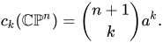
{\displaystyle c_{k}(\mathbb {C} \mathbb {P} ^{n})={\binom {n+1}{k}}a^{k}.}
チャーン多項式 チャーン多項式は、チャーン類と関連する概念を体系的に扱うのに便利な方法です。定義により、複素ベクトル束 E に対して、 E の チャーン多項式 c t は 次のように表されます。
c
t
(
E
)
=
1
+
c
1
(
E
)
t
+
⋯
+
c
n
(
E
)
t
n
.
{\displaystyle c_{t}(E)=1+c_{1}(E)t+\cdots +c_{n}(E)t^{n}.}
これは新しい不変量ではありません。形式変数 tは単に c k ( E )の次数を追跡するだけです 。 [6] 特に、は E の 全チャーン類 によって完全に決定されます 。 そしてその逆も同様です。
c
t
(
E
)
{\displaystyle c_{t}(E)}
c
(
E
)
=
1
+
c
1
(
E
)
+
⋯
+
c
n
(
E
)
{\displaystyle c(E)=1+c_{1}(E)+\cdots +c_{n}(E)}
チャーン類の公理の 1 つであるホイットニーの和の公式 (下記参照) によれば、 c t は次 のような意味で加法的である。
さて、 が (複素) 直線束の直和である場合、和の公式から次のことが導かれる。 ここで、
は最初のチャーン類である。 E の チャーン根 と呼ばれる 根は 、多項式の係数を決定する。すなわち、
σ k は 基本対称多項式 である 。 言い換えれば、 a i を 形式変数と考えると、 c k は「σ k である」 。 対称多項式 に関する基本的な事実は、たとえば t i の任意の対称多項式は、 t i の基本対称多項式の多項式であるということである 。 分割原理 または環理論のいずれかによって、任意のチャーン多項式は、 コホモロジー環を拡大した後、線形因子に因数分解される。前述の議論では、 E は 直線束の直和である必要はない。 結論は次のようになる。
c
t
(
E
⊕
E
′
)
=
c
t
(
E
)
c
t
(
E
′
)
.
{\displaystyle c_{t}(E\oplus E')=c_{t}(E)c_{t}(E').}
E
=
L
1
⊕
⋯
⊕
L
n
{\displaystyle E=L_{1}\oplus \cdots \oplus L_{n}}
c
t
(
E
)
=
(
1
+
a
1
(
E
)
t
)
⋯
(
1
+
a
n
(
E
)
t
)
{\displaystyle c_{t}(E)=(1+a_{1}(E)t)\cdots (1+a_{n}(E)t)}
a
i
(
E
)
=
c
1
(
L
i
)
{\displaystyle a_{i}(E)=c_{1}(L_{i})}
a
i
(
E
)
{\displaystyle a_{i}(E)}
c
k
(
E
)
=
σ
k
(
a
1
(
E
)
,
…
,
a
n
(
E
)
)
{\displaystyle c_{k}(E)=\sigma _{k}(a_{1}(E),\ldots ,a_{n}(E))}
c
t
(
E
)
{\displaystyle c_{t}(E)}
「複素ベクトル束 E における任意の対称多項式 f を評価するには、 f をσ k の多項式として 書き 、 σ k を c k ( E )に置き換えます 。」
例 :などの
多項式 s k が あります( ニュートンの恒等式 を参照)。この和は
E
のチャーン指標と呼ばれ 、最初の数項は次のようになります ( E は 省略します)。
t
1
k
+
⋯
+
t
n
k
=
s
k
(
σ
1
(
t
1
,
…
,
t
n
)
,
…
,
σ
k
(
t
1
,
…
,
t
n
)
)
{\displaystyle t_{1}^{k}+\cdots +t_{n}^{k}=s_{k}(\sigma _{1}(t_{1},\ldots ,t_{n}),\ldots ,\sigma _{k}(t_{1},\ldots ,t_{n}))}
s
1
=
σ
1
,
s
2
=
σ
1
2
−
2
σ
2
{\displaystyle s_{1}=\sigma _{1},s_{2}=\sigma _{1}^{2}-2\sigma _{2}}
ch
(
E
)
=
e
a
1
(
E
)
+
⋯
+
e
a
n
(
E
)
=
∑
s
k
(
c
1
(
E
)
,
…
,
c
n
(
E
)
)
/
k
!
{\displaystyle \operatorname {ch} (E)=e^{a_{1}(E)}+\cdots +e^{a_{n}(E)}=\sum s_{k}(c_{1}(E),\ldots ,c_{n}(E))/k!}
ch
(
E
)
=
rk
+
c
1
+
1
2
(
c
1
2
−
2
c
2
)
+
1
6
(
c
1
3
−
3
c
1
c
2
+
3
c
3
)
+
⋯
.
{\displaystyle \operatorname {ch} (E)=\operatorname {rk} +c_{1}+{\frac {1}{2}}(c_{1}^{2}-2c_{2})+{\frac {1}{6}}(c_{1}^{3}-3c_{1}c_{2}+3c_{3})+\cdots .}
例 : E の トッド類は 次のように与えられます。
td
(
E
)
=
∏
1
n
a
i
1
−
e
−
a
i
=
1
+
1
2
c
1
+
1
12
(
c
1
2
+
c
2
)
+
⋯
.
{\displaystyle \operatorname {td} (E)=\prod _{1}^{n}{a_{i} \over 1-e^{-a_{i}}}=1+{1 \over 2}c_{1}+{1 \over 12}(c_{1}^{2}+c_{2})+\cdots .}
注 : チャーン類は本質的には初等対称多項式であるという観察は、チャーン類を「定義」するために使用できます。G n を n 次元複素ベクトル空間の無限グラスマン多項式とします 。 この 空間 に は 、階数のトートロジーベクトルバンドル 、つまりが備えられています 。 は、 階数ベクトルバンドルの 分類空間 と呼ばれます。これは、 X 上の 階数 n の任意の複素ベクトルバンドル E が 与えられたときに、 に沿った へ
の引き戻しが に同型となるような 連続写像が存在し
、この写像は ホモトピーを除いて一意であるためです。 ボレルの定理によれば、 G n のコホモロジー環は、初等対称多項式 σ k の多項式である対称多項式の環とまったく同じです。したがって、 f E の引き戻しは次の ようになります。
次に、次の式を代入します。
n
{\displaystyle n}
E
n
→
G
n
{\displaystyle E_{n}\to G_{n}}
G
n
{\displaystyle G_{n}}
n
{\displaystyle n}
f
E
:
X
→
G
n
{\displaystyle f_{E}:X\to G_{n}}
E
n
{\displaystyle E_{n}}
X
{\displaystyle X}
f
E
{\displaystyle f_{E}}
E
{\displaystyle E}
f
E
{\displaystyle f_{E}}
f
E
∗
:
Z
[
σ
1
,
…
,
σ
n
]
→
H
∗
(
X
,
Z
)
.
{\displaystyle f_{E}^{*}:\mathbb {Z} [\sigma _{1},\ldots ,\sigma _{n}]\to H^{*}(X,\mathbb {Z} ).}
c
k
(
E
)
=
f
E
∗
(
σ
k
)
.
{\displaystyle c_{k}(E)=f_{E}^{*}(\sigma _{k}).}
注意 : 任意の特性類はチャーン類の多項式である。理由は次の通りである。 を反変関手とし、CW 複体 Xに、 X 上の階数 n の複素ベクトル束の同型類の集合を割り当て 、写像にその引き戻しを割り当てるものとする。定義により、 特性類は からコホモロジー関手へ の自然変換である。 特性類は、コホモロジー環の環構造により環を形成する。 米田の補題によれば、この特性類の環は G n のコホモロジー環とまったく同じである 。
Vect
n
C
{\displaystyle \operatorname {Vect} _{n}^{\mathbb {C} }}
Vect
n
C
=
[
−
,
G
n
]
{\displaystyle \operatorname {Vect} _{n}^{\mathbb {C} }=[-,G_{n}]}
H
∗
(
−
,
Z
)
.
{\displaystyle H^{*}(-,\mathbb {Z} ).}
Nat
(
[
−
,
G
n
]
,
H
∗
(
−
,
Z
)
)
=
H
∗
(
G
n
,
Z
)
=
Z
[
σ
1
,
…
,
σ
n
]
.
{\displaystyle \operatorname {Nat} ([-,G_{n}],H^{*}(-,\mathbb {Z} ))=H^{*}(G_{n},\mathbb {Z} )=\mathbb {Z} [\sigma _{1},\ldots ,\sigma _{n}].}
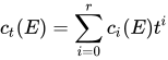
E を階数 r のベクトル束 と そのチャーン多項式
と します。
c
t
(
E
)
=
∑
i
=
0
r
c
i
(
E
)
t
i
{\displaystyle c_{t}(E)=\sum _{i=0}^{r}c_{i}(E)t^{i}}
の 双対バンドル については 、 . [7]
E
∗
{\displaystyle E^{*}}
E
{\displaystyle E}
c
i
(
E
∗
)
=
(
−
1
)
i
c
i
(
E
)
{\displaystyle c_{i}(E^{*})=(-1)^{i}c_{i}(E)}
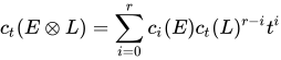
L が線束 ならば [8] [9] で あり、
c
t
(
E
⊗
L
)
=
∑
i
=
0
r
c
i
(
E
)
c
t
(
L
)
r
−
i
t
i
{\displaystyle c_{t}(E\otimes L)=\sum _{i=0}^{r}c_{i}(E)c_{t}(L)^{r-i}t^{i}}
c
i
(
E
⊗
L
)
,
i
=
1
,
2
,
…
,
r
{\displaystyle c_{i}(E\otimes L),i=1,2,\dots ,r}
c
1
(
E
)
+
r
c
1
(
L
)
,
…
,
∑
j
=
0
i
(
r
−
i
+
j
j
)
c
i
−
j
(
E
)
c
1
(
L
)
j
,
…
,
∑
j
=
0
r
c
r
−
j
(
E
)
c
1
(
L
)
j
.
{\displaystyle c_{1}(E)+rc_{1}(L),\dots ,\sum _{j=0}^{i}{\binom {r-i+j}{j}}c_{i-j}(E)c_{1}(L)^{j},\dots ,\sum _{j=0}^{r}c_{r-j}(E)c_{1}(L)^{j}.}
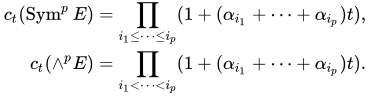
の チャーン根については 、 [10] 特に、
α
1
,
…
,
α
r
{\displaystyle \alpha _{1},\dots ,\alpha _{r}}
E
{\displaystyle E}
c
t
(
Sym
p
E
)
=
∏
i
1
≤
⋯
≤
i
p
(
1
+
(
α
i
1
+
⋯
+
α
i
p
)
t
)
,
c
t
(
∧
p
E
)
=
∏
i
1
<
⋯
<
i
p
(
1
+
(
α
i
1
+
⋯
+
α
i
p
)
t
)
.
{\displaystyle {\begin{aligned}c_{t}(\operatorname {Sym} ^{p}E)&=\prod _{i_{1}\leq \cdots \leq i_{p}}(1+(\alpha _{i_{1}}+\cdots +\alpha _{i_{p}})t),\\c_{t}(\wedge ^{p}E)&=\prod _{i_{1}<\cdots <i_{p}}(1+(\alpha _{i_{1}}+\cdots +\alpha _{i_{p}})t).\end{aligned}}}
c
1
(
∧
r
E
)
=
c
1
(
E
)
.
{\displaystyle c_{1}(\wedge ^{r}E)=c_{1}(E).}
例えば、 [11] では 、
c
i
=
c
i
(
E
)
{\displaystyle c_{i}=c_{i}(E)}
いつ 、
r
=
2
{\displaystyle r=2}
c
(
Sym
2
E
)
=
1
+
3
c
1
+
2
c
1
2
+
4
c
2
+
4
c
1
c
2
,
{\displaystyle c(\operatorname {Sym} ^{2}E)=1+3c_{1}+2c_{1}^{2}+4c_{2}+4c_{1}c_{2},}
いつ 、
r
=
3
{\displaystyle r=3}
c
(
Sym
2
E
)
=
1
+
4
c
1
+
5
c
1
2
+
5
c
2
+
2
c
1
3
+
11
c
1
c
2
+
7
c
3
.
{\displaystyle c(\operatorname {Sym} ^{2}E)=1+4c_{1}+5c_{1}^{2}+5c_{2}+2c_{1}^{3}+11c_{1}c_{2}+7c_{3}.}
(cf. Segre クラス#例 2 )
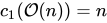
これらの抽象プロパティを使用して、 上の線束の残りのチャーン類を計算できます 。 を 示したことを思い出してください 。次に、テンソルの累乗を使用して、任意の整数に対する のチャーン類に関連付けることができます 。
C
P
1
{\displaystyle \mathbb {CP} ^{1}}
O
(
−
1
)
∗
≅
O
(
1
)
{\displaystyle {\mathcal {O}}(-1)^{*}\cong {\mathcal {O}}(1)}
c
1
(
O
(
1
)
)
=
1
∈
H
2
(
C
P
1
;
Z
)
{\displaystyle c_{1}({\mathcal {O}}(1))=1\in H^{2}(\mathbb {CP} ^{1};\mathbb {Z} )}
c
1
(
O
(
n
)
)
=
n
{\displaystyle c_{1}({\mathcal {O}}(n))=n}
プロパティ 位相空間 X 上の 複素ベクトル束 E が与えられたとき 、 Eのチャーン類は X の コホモロジー の元の列である 。 E の k 番目のチャーン類は c k ( E )と表記され、 整数 係数を持つ X
のコホモロジー の元である
。また、 全チャーン類 を定義することもできる。
H
2
k
(
X
;
Z
)
,
{\displaystyle H^{2k}(X;\mathbb {Z} ),}
c
(
E
)
=
c
0
(
E
)
+
c
1
(
E
)
+
c
2
(
E
)
+
⋯
.
{\displaystyle c(E)=c_{0}(E)+c_{1}(E)+c_{2}(E)+\cdots .}
値は実係数のコホモロジーではなく整数コホモロジー群にあるため、これらのチャーン類はリーマンの例のものよりもわずかに洗練されています。 [ 説明が必要 ]
古典的な公理的定義 チャーン類は次の 4 つの公理を満たします。
c
0
(
E
)
=
1
{\displaystyle c_{0}(E)=1}
すべてのE について 。 自然性: が 連続 で、 f*E が E の ベクトル束の引き戻し である場合 、 となります 。
f
:
Y
→
X
{\displaystyle f:Y\to X}
c
k
(
f
∗
E
)
=
f
∗
c
k
(
E
)
{\displaystyle c_{k}(f^{*}E)=f^{*}c_{k}(E)}
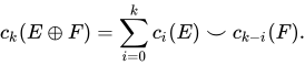
ホイットニー 和公式: が別の複素ベクトル束である場合、 直和 のチャーン類は 次の ように与えられる。
F
→
X
{\displaystyle F\to X}
E
⊕
F
{\displaystyle E\oplus F}
c
(
E
⊕
F
)
=
c
(
E
)
⌣
c
(
F
)
;
{\displaystyle c(E\oplus F)=c(E)\smile c(F);}
c
k
(
E
⊕
F
)
=
∑
i
=
0
k
c
i
(
E
)
⌣
c
k
−
i
(
F
)
.
{\displaystyle c_{k}(E\oplus F)=\sum _{i=0}^{k}c_{i}(E)\smile c_{k-i}(F).}
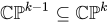
正規化:上の トートロジー直線束 の全チャーン類は 1− H であり、ここで H は 超平面 の ポアンカレ双対で ある。
C
P
k
{\displaystyle \mathbb {CP} ^{k}}
C
P
k
−
1
⊆
C
P
k
{\displaystyle \mathbb {CP} ^{k-1}\subseteq \mathbb {CP} ^{k}}
グロタンディークの公理的アプローチ あるいは、 アレクサンダー・グロタンディーク (1958) は、これらをわずかに小さい公理のセットに置き換えました。
自然度: (上記と同じ) 加法性: が ベクトル束の 正確な列 である場合、 です 。
0
→
E
′
→
E
→
E
″
→
0
{\displaystyle 0\to E'\to E\to E''\to 0}
c
(
E
)
=
c
(
E
′
)
⌣
c
(
E
″
)
{\displaystyle c(E)=c(E')\smile c(E'')}
正規化: E が 線束 である場合 、 は 基礎となる実ベクトル束の オイラー類 です 。
c
(
E
)
=
1
+
e
(
E
R
)
{\displaystyle c(E)=1+e(E_{\mathbb {R} })}
e
(
E
R
)
{\displaystyle e(E_{\mathbb {R} })}
彼は、ルレイ・ヒルシュの定理 を用いて 、任意の有限階数の複素ベクトル束の全チャーン類が、トートロジー的に定義された直線束の最初のチャーン類によって定義できることを示しています。
つまり、階数 n の 複素ベクトル束 E → B の射影化を、 任意の点における繊維が 繊維 E b の射影空間であるB 上の繊維束として導入する 。この束の全空間には 、 と表記する同義複素直線束が備わり、 第 1 チャーン類は、
複素射影空間 のコホモロジーを考慮して、繊維のコホモロジーを張る超平面の (ポアンカレ双対) 類をマイナスして、
各繊維に対して に制限します 。
P
(
E
)
{\displaystyle \mathbb {P} (E)}
b
∈
B
{\displaystyle b\in B}
P
(
E
)
{\displaystyle \mathbb {P} (E)}
τ
{\displaystyle \tau }
c
1
(
τ
)
=:
−
a
{\displaystyle c_{1}(\tau )=:-a}
P
(
E
b
)
{\displaystyle \mathbb {P} (E_{b})}
したがって、クラスは、
ファイバーのコホモロジーの基底に制限されるアンビエントコホモロジークラスの族を形成します。Leray -Hirsch の定理は 、 の任意のクラスは、基底上のクラスを係数として、 1、 a 、 a 2 、...、 a n −1 の線形結合として一意に表すことができることを述べています 。
1
,
a
,
a
2
,
…
,
a
n
−
1
∈
H
∗
(
P
(
E
)
)
{\displaystyle 1,a,a^{2},\ldots ,a^{n-1}\in H^{*}(\mathbb {P} (E))}
H
∗
(
P
(
E
)
)
{\displaystyle H^{*}(\mathbb {P} (E))}
特に、 グロタンディークの意味で E のチャーン類を定義することができ、これはクラス を次の 関係式で拡張することによって表される。
c
1
(
E
)
,
…
c
n
(
E
)
{\displaystyle c_{1}(E),\ldots c_{n}(E)}
−
a
n
{\displaystyle -a^{n}}
−
a
n
=
c
1
(
E
)
⋅
a
n
−
1
+
⋯
+
c
n
−
1
(
E
)
⋅
a
+
c
n
(
E
)
.
{\displaystyle -a^{n}=c_{1}(E)\cdot a^{n-1}+\cdots +c_{n-1}(E)\cdot a+c_{n}(E).}
次に、この代替定義が、自分が好む他の定義と一致するかどうかを確認したり、以前の公理的な特徴付けを使用したりすることができます。
チャーンクラスのトップ 実際、これらのプロパティはチャーン類を独自に特徴づけます。それらは、とりわけ次のことを意味します。
n が V の複素階数である 場合 、すべての k > n に対して 成り立ちます。したがって、全体のチャーン類は終了します。
c
k
(
V
)
=
0
{\displaystyle c_{k}(V)=0}
V の上位チャーン類 (つまり 、 nは V の階数)は、常に 基礎となる実ベクトル束の オイラー類 に等しい。
c
n
(
V
)
{\displaystyle c_{n}(V)}
代数幾何学では
公理的な説明 コホモロジー環の代数幾何的な類似体であるチョウ環の値を取るチャーン類の別の構成もあり ます 。
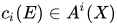
を次元 の非特異な準射影多様体と する。チャーン類と呼ばれる 要素に代数的ベクトル束を割り当て 、チャーン多項式 を 満たす唯一のチャーン類理論が存在し、次の式を満たすことが示される (グロタンディークの公理的アプローチに類似)。 [12]
X
{\displaystyle X}
n
{\displaystyle n}
E
→
X
{\displaystyle E\to X}
c
i
(
E
)
∈
A
i
(
X
)
{\displaystyle c_{i}(E)\in A^{i}(X)}
c
t
(
E
)
=
c
0
(
E
)
+
c
1
(
E
)
t
+
⋯
+
c
n
(
E
)
t
n
{\displaystyle c_{t}(E)=c_{0}(E)+c_{1}(E)t+\cdots +c_{n}(E)t^{n}}
カルティエ因子 の場合 、 となり 、 となります 。
D
{\displaystyle D}
E
≅
O
X
(
D
)
{\displaystyle E\cong {\mathcal {O}}_{X}(D)}
c
t
(
E
)
=
1
+
D
t
{\displaystyle c_{t}(E)=1+Dt}
が射なら ば、 です 。
f
:
X
′
→
X
{\displaystyle f:X'\to X}
c
i
(
f
∗
E
)
=
f
∗
c
i
(
E
)
{\displaystyle c_{i}(f^{*}E)=f^{*}c_{i}(E)}
が上のベクトル束の正確な列である 場合 、ホイットニーの和の公式が成り立ちます 。
0
→
E
′
→
E
→
E
″
→
0
{\displaystyle 0\to E'\to E\to E''\to 0}
X
{\displaystyle X}
c
t
(
E
)
=
c
t
(
E
′
)
c
t
(
E
″
)
{\displaystyle c_{t}(E)=c_{t}(E')c_{t}(E'')}
通常のシーケンス 射影空間の特性類を計算することは、多くの特性類計算の基礎となる。なぜなら、任意の滑らかな射影部分多様体に対して、 短い完全列が存在するからである。
X
⊂
P
n
{\displaystyle X\subset \mathbb {P} ^{n}}
0
→
T
X
→
T
P
n
|
X
→
N
X
/
P
n
→
0
{\displaystyle 0\to {\mathcal {T}}_{X}\to {\mathcal {T}}_{\mathbb {P} ^{n}}|_{X}\to {\mathcal {N}}_{X/\mathbb {P} ^{n}}\to 0}
五次三重 例えば、 の非特異 五次三次 多様体を考える 。その正規束は で与えられ 、短完全列
P
4
{\displaystyle \mathbb {P} ^{4}}
O
X
(
5
)
{\displaystyle {\mathcal {O}}_{X}(5)}
0
→
T
X
→
T
P
4
|
X
→
O
X
(
5
)
→
0
{\displaystyle 0\to {\mathcal {T}}_{X}\to {\mathcal {T}}_{\mathbb {P} ^{4}}|_{X}\to {\mathcal {O}}_{X}(5)\to 0}
における超平面類を と表す と、ホイットニーの和の公式は次式を与える。
h
{\displaystyle h}
A
∙
(
X
)
{\displaystyle A^{\bullet }(X)}
c
(
T
X
)
c
(
O
X
(
5
)
)
=
(
1
+
h
)
5
=
1
+
5
h
+
10
h
2
+
10
h
3
{\displaystyle c({\mathcal {T}}_{X})c({\mathcal {O}}_{X}(5))=(1+h)^{5}=1+5h+10h^{2}+10h^{3}}
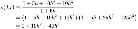
超曲面のチャウ環を計算するのは難しいので、この列を の連接層の列として考えることにする 。これにより、
P
4
{\displaystyle \mathbb {P} ^{4}}
c
(
T
X
)
=
1
+
5
h
+
10
h
2
+
10
h
3
1
+
5
h
=
(
1
+
5
h
+
10
h
2
+
10
h
3
)
(
1
−
5
h
+
25
h
2
−
125
h
3
)
=
1
+
10
h
2
−
40
h
3
{\displaystyle {\begin{aligned}c({\mathcal {T}}_{X})&={\frac {1+5h+10h^{2}+10h^{3}}{1+5h}}\\&=\left(1+5h+10h^{2}+10h^{3}\right)\left(1-5h+25h^{2}-125h^{3}\right)\\&=1+10h^{2}-40h^{3}\end{aligned}}}
ガウス・ボネの定理を使用して、クラスを積分して オイラー特性を計算することができます。伝統的に、これはオイラー クラス と呼ばれます。これは、
クラスが5 つの点 ( ベズーの定理 による) で表すことができるためです。オイラー特性は 、オイラー特性の定義とレフシェッツの超平面定理を使用して、
コホモロジーのベッティ数を計算するために使用できます。
c
3
(
T
X
)
{\displaystyle c_{3}({\mathcal {T}}_{X})}
∫
[
X
]
c
3
(
T
X
)
=
∫
[
X
]
−
40
h
3
=
−
200
{\displaystyle \int _{[X]}c_{3}({\mathcal {T}}_{X})=\int _{[X]}-40h^{3}=-200}
h
3
{\displaystyle h^{3}}
X
{\displaystyle X}
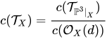
d次超曲面 が 次滑らかな超曲面である 場合、 関係式を与える 短い正確な数列が得られ 、これを として計算して、
全チャーン類を与えることができます。特に、 が偶数である 場合は がスピン 4 多様体であること
が分かる ので、 次 の滑らかな超曲面はすべて スピン多様体 です 。
X
⊂
P
3
{\displaystyle X\subset \mathbb {P} ^{3}}
d
{\displaystyle d}
0
→
T
X
→
T
P
3
|
X
→
O
X
(
d
)
→
0
{\displaystyle 0\to {\mathcal {T}}_{X}\to {\mathcal {T}}_{\mathbb {P} ^{3}}|_{X}\to {\mathcal {O}}_{X}(d)\to 0}
c
(
T
X
)
=
c
(
T
P
3
|
X
)
c
(
O
X
(
d
)
)
{\displaystyle c({\mathcal {T}}_{X})={\frac {c({\mathcal {T}}_{\mathbb {P} ^{3}|_{X}})}{c({\mathcal {O}}_{X}(d))}}}
c
(
T
X
)
=
(
1
+
[
H
]
)
4
(
1
+
d
[
H
]
)
=
(
1
+
4
[
H
]
+
6
[
H
]
2
)
(
1
−
d
[
H
]
+
d
2
[
H
]
2
)
=
1
+
(
4
−
d
)
[
H
]
+
(
6
−
4
d
+
d
2
)
[
H
]
2
{\displaystyle {\begin{aligned}c({\mathcal {T}}_{X})&={\frac {(1+[H])^{4}}{(1+d[H])}}\\&=(1+4[H]+6[H]^{2})(1-d[H]+d^{2}[H]^{2})\\&=1+(4-d)[H]+(6-4d+d^{2})[H]^{2}\end{aligned}}}
X
{\displaystyle X}
4
−
d
{\displaystyle 4-d}
2
k
{\displaystyle 2k}
近似概念
チャーンキャラクター チャーン類は、空間の位相的K理論 からその有理コホモロジー(の完備化)への環の準同型を構成するために使用できる 。直線束 L に対して、チャーン指標chは次のように定義される。
ch
(
L
)
=
exp
(
c
1
(
L
)
)
:=
∑
m
=
0
∞
c
1
(
L
)
m
m
!
.
{\displaystyle \operatorname {ch} (L)=\exp(c_{1}(L)):=\sum _{m=0}^{\infty }{\frac {c_{1}(L)^{m}}{m!}}.}
より一般的には、 直線束の直和の場合、第一チャーン類を用いて チャーン指標は加法的に定義される。
V
=
L
1
⊕
⋯
⊕
L
n
{\displaystyle V=L_{1}\oplus \cdots \oplus L_{n}}
x
i
=
c
1
(
L
i
)
,
{\displaystyle x_{i}=c_{1}(L_{i}),}
ch
(
V
)
=
e
x
1
+
⋯
+
e
x
n
:=
∑
m
=
0
∞
1
m
!
(
x
1
m
+
⋯
+
x
n
m
)
.
{\displaystyle \operatorname {ch} (V)=e^{x_{1}}+\cdots +e^{x_{n}}:=\sum _{m=0}^{\infty }{\frac {1}{m!}}(x_{1}^{m}+\cdots +x_{n}^{m}).}
これは次のように書き直すことができる: [13]
ch
(
V
)
=
rk
(
V
)
+
c
1
(
V
)
+
1
2
(
c
1
(
V
)
2
−
2
c
2
(
V
)
)
+
1
6
(
c
1
(
V
)
3
−
3
c
1
(
V
)
c
2
(
V
)
+
3
c
3
(
V
)
)
+
⋯
.
{\displaystyle \operatorname {ch} (V)=\operatorname {rk} (V)+c_{1}(V)+{\frac {1}{2}}(c_{1}(V)^{2}-2c_{2}(V))+{\frac {1}{6}}(c_{1}(V)^{3}-3c_{1}(V)c_{2}(V)+3c_{3}(V))+\cdots .}
この最後の表現は、 分割原理 を適用することで正当化され、任意のベクトル束 V の定義 ch(V) として解釈されます。
基底が多様体であるときに接続を使用してチャーン類を定義する場合(つまり、 チャーン-ヴェイユ理論 )、チャーン指標の明示的な形式は次のようになります
。ここで、 Ω は接続の
曲率 です。
ch
(
V
)
=
[
tr
(
exp
(
i
Ω
2
π
)
)
]
{\displaystyle \operatorname {ch} (V)=\left[\operatorname {tr} \left(\exp \left({\frac {i\Omega }{2\pi }}\right)\right)\right]}
チャーン キャラクタは、テンソル積のチャーン クラスの計算を容易にするため、便利です。具体的には、次の恒等式に従います。
ch
(
V
⊕
W
)
=
ch
(
V
)
+
ch
(
W
)
{\displaystyle \operatorname {ch} (V\oplus W)=\operatorname {ch} (V)+\operatorname {ch} (W)}
ch
(
V
⊗
W
)
=
ch
(
V
)
ch
(
W
)
.
{\displaystyle \operatorname {ch} (V\otimes W)=\operatorname {ch} (V)\operatorname {ch} (W).}
上で述べたように、チャーン類のグロタンディーク加法公理を使用すると、これらの 恒等式の最初のものは一般化されて、 chは K 理論 K ( X )から X の有理コホモロジーへのアーベル群 の 準同型 であると述べることができます。2 番目の恒等式は、この準同型が K ( X )の積も尊重するという事実を確立し 、したがって ch は 環の準同型です。
チャーン指標は ヒルツェブルッフ・リーマン・ロッホの定理 で使用されます。
チャーン数 次元 の 有向多様 体で作業する場合 、全次数 のチャーン類の積 (つまり、積内のチャーン類のインデックスの合計は になる)は、 方向ホモロジー類 と組み合わせる (または「多様体上で積分する」)ことで整数、つまりベクトル束の チャーン数 を得ることができます。たとえば、多様体の次元が 6 の場合、 、 、 で示される 3 つの線形独立なチャーン数が存在します 。 一般 に、多様体の次元が の場合 、可能な独立なチャーン数の数は の 分割 数です。
2
n
{\displaystyle 2n}
2
n
{\displaystyle 2n}
n
{\displaystyle n}
c
1
3
{\displaystyle c_{1}^{3}}
c
1
c
2
{\displaystyle c_{1}c_{2}}
c
3
{\displaystyle c_{3}}
2
n
{\displaystyle 2n}
n
{\displaystyle n}
複素数(またはほぼ複素数)多様体の接束のチャーン数は多様体のチャーン数と呼ばれ、重要な不変量です。
一般化されたコホモロジー理論 チャーン類の理論の一般化があり、通常のコホモロジーが 一般化されたコホモロジー理論 に置き換えられます。このような一般化が可能な理論は、 複素有向 と呼ばれます。チャーン類の形式的な性質は同じままですが、重要な違いが 1 つあります。それは、因子の最初のチャーン類に関して直線束のテンソル積の最初のチャーン類を計算する規則は、(通常の) 加算ではなく、 形式的な群法則 であるということです。
代数幾何学 代数幾何学には、ベクトル束のチャーン類の同様の理論があります。チャーン類がどのグループに属するかによって、いくつかのバリエーションがあります。
複素多様体の場合、チャーン類は上記のように通常のコホモロジー内の値を取ることができます。 一般体上の多様体の場合、チャーン類は エタールコホモロジー や l 進コホモロジー などのコホモロジー理論で値を取ることができます。 一般体上の多様体 V に対して、チャーン類は チョウ群 CH(V) の準同型で値を取ることもできます。たとえば、多様体 V 上の直線束の最初のチャーン類は、次数を 1 減らすCH( V ) から CH( V ) への準同型です。これは、チョウ群がホモロジー群の一種の類似体であり、コホモロジー群の元は キャップ積 を使用するホモロジー群の準同型として考えることができるという事実に対応します 。
構造を持つ多様体 チャーン類の理論は、 ほぼ複素多様体 に対する コボルディズム 不変量を生み出します。
M が概複素多様体である 場合、その 接束は 複素ベクトル束である。したがって、 M の チャーン類は 、その接束のチャーン類として定義される。 M も コンパクト で次元が 2 d である場合、チャーン類の 全次数 2 d の各 単項式は、 M の 基本類 とペアにすることができ、整数、つまり M の チャーン数を 与える。 M ′ が同じ次元の別の概複素多様体である場合、 M ′のチャーン数が M のチャーン数と一致する場合のみ、 M は M と共形である 。
この理論は、互換性のあるほぼ複素構造を介することで、実 シンプレク ティック ベクトル束にも拡張されます。特に、 シンプレクティック多様体は 明確に定義されたチャーン類を持ちます。
算術スキームとディオファントス方程式 ( アラケロフ幾何学を 参照)
参照
注記
^ ボット、ラウル 、トゥ、ローリング(1995年)。 代数的位相幾何学における微分形式 (Corr. 3.印刷版)。ニューヨーク[ua]:シュプリンガー。p. 267ff。ISBN 3-540-90613-4 。 ^ Hatcher, Allen . 「ベクトル束とK理論」 (PDF) 命題3.10。 ^ 編集者注: 私たちの表記法はMilnor−Stasheffとは異なりますが、より自然に思われます。 ^ この数列は オイラー数列 と呼ばれることもあります。 ^ Hartshorne、第II章、定理8.13。 ^ 環論の項では、次数付き環の同型が存在します。
ここで、左辺は偶数項のコホモロジー環、η は次数を無視した環準同型であり、 xは同次で次数 | x |を持ちます 。
H
2
∗
(
M
,
Z
)
→
⊕
k
∞
η
(
H
2
∗
(
M
,
Z
)
)
[
t
]
,
x
↦
x
t
|
x
|
/
2
{\displaystyle H^{2*}(M,\mathbb {Z} )\to \oplus _{k}^{\infty }\eta (H^{2*}(M,\mathbb {Z} ))[t],x\mapsto xt^{|x|/2}}
^ フルトン、注釈3.2.3. (a) ^ フルトン、注釈3.2.3. (b) ^ Fulton、例3.2.2。 ^ フルトン、注釈3.2.3. (c) ^ たとえば、WolframAlpha を使用して多項式を展開し、 が 基本的な対称多項式であるという事実を使用します 。
c
i
{\displaystyle c_{i}}
α
i
{\displaystyle \alpha _{i}}
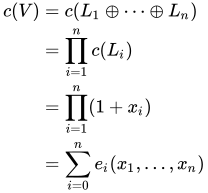
^ Hartshorne、付録A. 3 Chern クラス。 ^ (§ チャーン多項式も参照) V が 線束の和であるとき、 V のチャーン類はにおける 基本対称多項式 として表現できることに注目してください。特に 、
一方では であり、
他方では
その結果、 ニュートンの恒等式を使用して、上記の ch( V )におけるべき乗和を V のチャーン類のみで再表現し 、主張する式を与えることができます。
x
i
{\displaystyle x_{i}}
c
i
(
V
)
=
e
i
(
x
1
,
…
,
x
n
)
.
{\displaystyle c_{i}(V)=e_{i}(x_{1},\ldots ,x_{n}).}
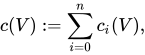
c
(
V
)
:=
∑
i
=
0
n
c
i
(
V
)
,
{\displaystyle c(V):=\sum _{i=0}^{n}c_{i}(V),}
c
(
V
)
=
c
(
L
1
⊕
⋯
⊕
L
n
)
=
∏
i
=
1
n
c
(
L
i
)
=
∏
i
=
1
n
(
1
+
x
i
)
=
∑
i
=
0
n
e
i
(
x
1
,
…
,
x
n
)
{\displaystyle {\begin{aligned}c(V)&=c(L_{1}\oplus \cdots \oplus L_{n})\\&=\prod _{i=1}^{n}c(L_{i})\\&=\prod _{i=1}^{n}(1+x_{i})\\&=\sum _{i=0}^{n}e_{i}(x_{1},\ldots ,x_{n})\end{aligned}}}
参考文献
外部リンク





![{\displaystyle \Omega =d\omega +{\frac {1}{2}}[\omega ,\omega ]}](https://wikimedia.org/api/rest_v1/media/math/render/svg/c2f7c4659b6e7352c32510a81c0d9f8afdeab74e)



![{\displaystyle \sum _{k}c_{k}(V)t^{k}=\left[I+i{\frac {\mathrm {tr} (\Omega )}{2\pi }}t+{ \frac {\mathrm {tr} (\Omega ^{2})-\mathrm {tr} (\Omega )^{2}}{8\pi ^{2}}}t^{2}+i{\frac {-2\mathrm {tr} (\Omega ^{3})+3\mathrm {tr} (\Omega ^{2})\mathrm { tr} (\Omega )-\mathrm {tr} (\Omega )^{3}}{48\pi ^{3}}}t^{3}+\cdots \right].}](https://wikimedia.org/api/rest_v1/media/math/render/svg/59c15f6af93ba119ded46890d1c02f1ba213f334)









![{\displaystyle c_{1}=\left[{\frac {i}{2\pi }}\operatorname {tr} \Omega \right].}](https://wikimedia.org/api/rest_v1/media/math/render/svg/55b51326e739a3dc716d0f6d9e0d5d095d6c3fe8)








































![{\displaystyle f_{E}^{*}:\mathbb {Z} [\sigma _{1},\ldots ,\sigma _{n}]\to H^{*}(X,\mathbb {Z} ).}](https://wikimedia.org/api/rest_v1/media/math/render/svg/01756308bbe78178bd49f25f1e5e2aa297e0c025)


![{\displaystyle \operatorname {Vect} _{n}^{\mathbb {C} }=[-,G_{n}]}](https://wikimedia.org/api/rest_v1/media/math/render/svg/a335e563799383694e3073de608043b248286367)

![{\displaystyle \operatorname {Nat} ([-,G_{n}],H^{*}(-,\mathbb {Z} ))=H^{*}(G_{n},\mathbb {Z} )=\mathbb {Z} [\sigma _{1},\ldots ,\sigma _{n}].}](https://wikimedia.org/api/rest_v1/media/math/render/svg/c796a5ea1c5c3e24fabeb95c5cfeef9d7c66150e)










































![{\displaystyle \int _{[X]}c_{3}({\mathcal {T}}_{X})=\int _{[X]}-40h^{3}=-200}](https://wikimedia.org/api/rest_v1/media/math/render/svg/1cc53a6bd8f1db3ed43036979c121c553109d53b)



![{\displaystyle {\begin{aligned}c({\mathcal {T}}_{X})&={\frac {(1+[H])^{4}}{(1+d[H])}}\\&=(1+4[H]+6[H]^{2})(1-d[H]+d^{2}[H]^{2})\\&=1+(4-d)[H]+(6-4d+d^{2})[H]^{2}\end{aligned}}}](https://wikimedia.org/api/rest_v1/media/math/render/svg/ca2779c48dbc64c5414a4da97c9f9941accadf3a)







![{\displaystyle \operatorname {ch} (V)=\left[\operatorname {tr} \left(\exp \left({\frac {i\Omega }{2\pi }}\right)\right)\right]}](https://wikimedia.org/api/rest_v1/media/math/render/svg/2473fa0b260fc2463468e8b3984a178804ba7ccf)




![{\displaystyle H^{2*}(M,\mathbb {Z} )\to \oplus _{k}^{\infty }\eta (H^{2*}(M,\mathbb {Z} ))[t],x\mapsto xt^{|x|/2}}](https://wikimedia.org/api/rest_v1/media/math/render/svg/2dd6eaeedff045ca1d0fe892e1e494984372baa2)