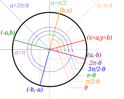
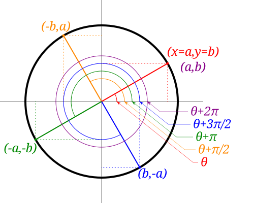
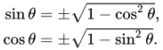
単位円を調べることで、三角関数の以下の性質を確立することができる。
兆候 三角関数の符号は角度の象限によって決まります。− π < θ ≤ π {\displaystyle {-\pi }<\theta \leq \pi } は 符号関数 です。
サイン ( 罪 θ ) = サイン ( csc θ ) = { + 1 もし 0 < θ < π − 1 もし − π < θ < 0 0 もし θ ∈ { 0 、 π } サイン ( コス θ ) = サイン ( 秒 θ ) = { + 1 もし − π 2 < θ < π 2 − 1 もし − π < θ < − π 2 または π 2 < θ < π 0 もし θ ∈ { − π 2 、 π 2 } サイン ( タン θ ) = サイン ( ベビーベッド θ ) = { + 1 もし − π < θ < − π 2 または 0 < θ < π 2 − 1 もし − π 2 < θ < 0 または π 2 < θ < π 0 もし θ ∈ { − π 2 、 0 、 π 2 、 π } {\displaystyle {\begin{aligned}\operatorname {sgn}(\sin \theta )=\operatorname {sgn}(\csc \theta )&={\begin{cases}+1&{\text{if}}\ \ 0<\theta <\pi \\-1&{\text{if}}\ \ {-\pi }<\theta <0\\0&{\text{if}}\ \ \theta \in \{0,\pi \}\end{cases}}\\[5mu]\operatorname {sgn}(\cos \theta )=\operatorname {sgn}(\sec \theta )&={\begin{cases}+1&{\text{if}}\ \ {-{\tfrac {\pi }{2}}}<\theta <{\tfrac {\pi }{2}}\\-1&{\text{if}}\ \ {-\pi }<\theta <-{\tfrac {\pi }{2}}\ \ {\text{or}}\ \ {\tfrac {\pi }{2}}<\theta <\pi \\0&{\text{if}}\ \ \theta \in {\bigl \{}{-{\tfrac {\pi }{2}}},{\tfrac {\pi }{2}}{\bigr \}}\end{cases}}\\[5mu]\operatorname {sgn}(\tan \theta )=\operatorname {sgn}(\cot \theta )&={\begin{cases}+1&{\text{if}}\ \ {-\pi }<\theta <-{\tfrac {\pi }{2}}\ \ {\text{or}}\ \ 0<\theta <{\tfrac {\pi }{2}}\\-1&{\text{if}}\ \ {-{\tfrac {\pi }{2}}}<\theta <0\ \ {\text{or}}\ \ {\tfrac {\pi }{2}}<\theta <\pi \\0&{\text{if}}\ \ \theta \in {\bigl \{}{-{\tfrac {\pi }{2}}},0,{\tfrac {\pi }{2}},\pi {\bigr \}}\end{cases}}\end{aligned}}}
三角関数は共通の周期を持つ周期関数である2 π 、 {\displaystyle 2\pi ,} θ の値が区間外の場合( − π 、 π ] 、 {\displaystyle ({-\pi },\pi ],} シフトと周期性」 の項 を参照)。正弦波または余弦波の符号を使用して、正規化された方形波 を定義できます。たとえば、関数サイン ( 罪 x ) {\displaystyle \operatorname {sgn}(\sin x)} サイン ( コス x ) {\displaystyle \operatorname {sgn}(\cos x)} 、位相シフトがπ / 2の 方形 波 。
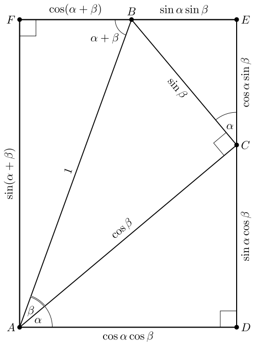
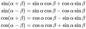
角度の和と差の公式 角度の和の三角関数の恒等式を導出するための幾何学的作図 角度差の公式を示す図罪 ( α − β ) {\displaystyle \sin(\alpha -\beta )} コス ( α − β ) {\displaystyle \cos(\alpha -\beta )} これらは角度の加法定理および減法定理 (または公式 ) としても知られています。罪 ( α + β ) = 罪 α コス β + コス α 罪 β 罪 ( α − β ) = 罪 α コス β − コス α 罪 β コス ( α + β ) = コス α コス β − 罪 α 罪 β コス ( α − β ) = コス α コス β + 罪 α 罪 β {\displaystyle {\begin{aligned}\sin(\alpha +\beta )&=\sin \alpha \cos \beta +\cos \alpha \sin \beta \\\sin(\alpha -\beta )&=\sin \alpha \cos \beta -\cos \alpha \sin \beta \\\cos(\alpha +\beta )&=\cos \alpha \cos \beta -\sin \alpha \sin \beta \\\cos(\alpha -\beta )&=\cos \alpha \cos \beta +\sin \alpha \sin \beta \end{aligned}}}
角度差の公式罪 ( α − β ) {\displaystyle \sin(\alpha -\beta )} コス ( α − β ) {\displaystyle \cos(\alpha -\beta )} − β {\displaystyle -\beta } β {\displaystyle \beta } 罪 ( − β ) = − 罪 ( β ) {\displaystyle \sin(-\beta )=-\sin(\beta )} コス ( − β ) = コス ( β ) {\displaystyle \cos(-\beta )=\cos(\beta )} も できます 。
これらの恒等式は、次の表の最初の2行にまとめられており、他の三角関数の和と差の恒等式も含まれています。
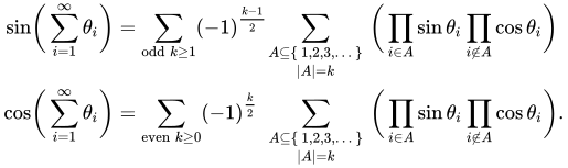
無限個の角度の和の正弦と余弦 シリーズが∑ 私 = 1 ∞ θ 私 \sum_{i=1}^{\infty}\theta_{i}} 収束する
罪 ( ∑ 私 = 1 ∞ θ 私 ) = ∑ 奇数 k ≥ 1 ( − 1 ) k − 1 2 ∑ A ⊆ { 1 、 2 、 3 、 … } | A | = k ( ∏ 私 ∈ A 罪 θ 私 ∏ 私 ∉ A コス θ 私 ) コス ( ∑ 私 = 1 ∞ θ 私 ) = ∑ 平 k ≥ 0 ( − 1 ) k 2 ∑ A ⊆ { 1 、 2 、 3 、 … } | A | = k ( ∏ 私 ∈ A 罪 θ 私 ∏ 私 ∉ A コス θ 私 ) 。 {\displaystyle {\begin{aligned}{\sin }{\biggl (}\sum _{i=1}^{\infty }\theta _{i}{\biggl )}&=\sum _{{\text{odd}}\ k\geq 1}(-1)^{\frac {k-1}{2}}\!\!\sum _{\begin{smallmatrix}A\subseteq \{\,1,2,3,\dots \,\}\\\left|A\right|=k\end{smallmatrix}}{\biggl (}\prod _{i\in A}\sin \theta _{i}\prod _{i\not \in A}\cos \theta _{i}{\biggr )}\\{\cos }{\biggl (}\sum _{i=1}^{\infty }\theta _{i}{\biggr )}&=\sum _{{\text{even}}\ k\geq 0}(-1)^{\frac {k}{2}}\,\sum _{\begin{smallmatrix}A\subseteq \{\,1,2,3,\dots \,\}\\\left|A\right|=k\end{smallmatrix}}{\biggl (}\prod _{i\in A}\sin \theta _{i}\prod _{i\not \in A}\cos \theta _{i}{\biggr )}.\end{aligned}}}
シリーズ∑ 私 = 1 ∞ θ 私 \sum_{i=1}^{\infty}\theta_{i}} リム 私 → ∞ θ 私 = 0 、 {\textstyle \lim _{i\to \infty }\theta _{i}=0,} リム 私 → ∞ 罪 θ 私 = 0 、 {\textstyle \lim _{i\to \infty }\sin \theta _{i}=0,} リム 私 → ∞ コス θ 私 = 1. {\textstyle \lim _{i\to \infty }\cos \theta _{i}=1.} 有限個しか ありません。正弦因子が無限個ある項は、必然的にゼロになります。
角度が有限個しかない場合θ 私 \displaystyle \theta _{i}}
和の正接と余接 させてe k {\displaystyle e_{k}} k = 0 、 1 、 2 、 3 、 … {\displaystyle k=0,1,2,3,\ldots } k 次基本対称多項式とする x 私 = タン θ 私 {\displaystyle x_{i}=\tan \theta _{i}} 私 = 0 、 1 、 2 、 3 、 … 、 {\displaystyle i=0,1,2,3,\ldots ,}
e 0 = 1 e 1 = ∑ 私 x 私 = ∑ 私 タン θ 私 e 2 = ∑ 私 < j x 私 x j = ∑ 私 < j タン θ 私 タン θ j e 3 = ∑ 私 < j < k x 私 x j x k = ∑ 私 < j < k タン θ 私 タン θ j タン θ k ⋮ ⋮ {\displaystyle {\begin{aligned}e_{0}&=1\\[6pt]e_{1}&=\sum _{i}x_{i}&&=\sum _{i}\tan \theta _{i}\\[6pt]e_{2}&=\sum _{i<j}x_{i}x_{j}&&=\sum _{i<j}\tan \theta _{i}\tan \theta _{j}\\[6pt]e_{3}&=\sum _{i<j<k}x_{i}x_{j}x_{k}&&=\sum _{i<j<k}\tan \theta _{i}\tan \theta _{j}\tan \theta _{k}\\&\ \ \vdots &&\ \ \vdots \end{aligned}}}
それから
タン ( ∑ 私 θ 私 ) = e 1 − e 3 + e 5 − ⋯ e 0 − e 2 + e 4 − ⋯ 。 {\displaystyle \tan {\Bigl (}\sum _{i}\theta _{i}{\Bigr )}={\frac {e_{1}-e_{3}+e_{5}-\cdots }{e_{0}-e_{2}+e_{4}-\cdots }}.} タン ( ∑ 私 θ 私 ) = 罪 ( ∑ 私 θ 私 ) / ∏ 私 コス θ 私 コス ( ∑ 私 θ 私 ) / ∏ 私 コス θ 私 = ∑ 奇数 k ≥ 1 ( − 1 ) k − 1 2 ∑ A ⊆ { 1 、 2 、 3 、 … } | A | = k ∏ 私 ∈ A タン θ 私 ∑ 平 k ≥ 0 ( − 1 ) k 2 ∑ A ⊆ { 1 、 2 、 3 、 … } | A | = k ∏ 私 ∈ A タン θ 私 = e 1 − e 3 + e 5 − ⋯ e 0 − e 2 + e 4 − ⋯ ベビーベッド ( ∑ 私 θ 私 ) = e 0 − e 2 + e 4 − ⋯ e 1 − e 3 + e 5 − ⋯ {\displaystyle {\begin{aligned}\tan {\Bigl (}\sum _{i}\theta _{i}{\Bigr )}&={\frac {{\sin }{\bigl (}\sum _{i}\theta _{i}{\bigr )}/\prod _{i}\cos \theta _{i}}{{\cos }{\bigl (}\sum _{i}\theta _{i}{\bigr )}/\prod _{i}\cos \theta _{i}}}\\[10pt]&={\frac {\displaystyle \sum _{{\text{odd}}\ k\geq 1}(-1)^{\frac {k-1}{2}}\sum _{\begin{smallmatrix}A\subseteq \{1,2,3,\dots \}\\\left|A\right|=k\end{smallmatrix}}\prod _{i\in A}\tan \theta _{i}}{\displaystyle \sum _{{\text{even}}\ k\geq 0}~(-1)^{\frac {k}{2}}~~\sum _{\begin{smallmatrix}A\subseteq \{1,2,3,\dots \}\\\left|A\right|=k\end{smallmatrix}}\prod _{i\in A}\tan \theta _{i}}}={\frac {e_{1}-e_{3}+e_{5}-\cdots }{e_{0}-e_{2}+e_{4}-\cdots }}\\[10pt]\cot {\Bigl (}\sum _{i}\theta _{i}{\Bigr )}&={\frac {e_{0}-e_{2}+e_{4}-\cdots }{e_{1}-e_{3}+e_{5}-\cdots }}\end{aligned}}}
右辺の項数は左辺の項数に依存する。
例えば: タン ( θ 1 + θ 2 ) = e 1 e 0 − e 2 = x 1 + x 2 1 − x 1 x 2 = タン θ 1 + タン θ 2 1 − タン θ 1 タン θ 2 、 タン ( θ 1 + θ 2 + θ 3 ) = e 1 − e 3 e 0 − e 2 = ( x 1 + x 2 + x 3 ) − ( x 1 x 2 x 3 ) 1 − ( x 1 x 2 + x 1 x 3 + x 2 x 3 ) 、 タン ( θ 1 + θ 2 + θ 3 + θ 4 ) = e 1 − e 3 e 0 − e 2 + e 4 = ( x 1 + x 2 + x 3 + x 4 ) − ( x 1 x 2 x 3 + x 1 x 2 x 4 + x 1 x 3 x 4 + x 2 x 3 x 4 ) 1 − ( x 1 x 2 + x 1 x 3 + x 1 x 4 + x 2 x 3 + x 2 x 4 + x 3 x 4 ) + ( x 1 x 2 x 3 x 4 ) 、 {\displaystyle {\begin{aligned}\tan(\theta _{1}+\theta _{2})&={\frac {e_{1}}{e_{0}-e_{2}}}={\frac {x_{1}+x_{2}}{1\ -\ x_{1}x_{2}}}={\frac {\tan \theta _{1}+\tan \theta _{2}}{1\ -\ \tan \theta _{1}\tan \theta _{2}}},\\[8pt]\tan(\theta _{1}+\theta _{2}+\theta _{3})&={\frac {e_{1}-e_{3}}{e_{0}-e_{2}}}={\frac {(x_{1}+x_{2}+x_{3})\ -\ (x_{1}x_{2}x_{3})}{1\ -\ (x_{1}x_{2}+x_{1}x_{3}+x_{2}x_{3})}},\\[8pt]\tan(\theta _{1}+\theta _{2}+\theta _{3}+\theta _{4})&={\frac {e_{1}-e_{3}}{e_{0}-e_{2}+e_{4}}}\\[8pt]&={\frac {(x_{1}+x_{2}+x_{3}+x_{4})\ -\ (x_{1}x_{2}x_{3}+x_{1}x_{2}x_{4}+x_{1}x_{3}x_{4}+x_{2}x_{3}x_{4})}{1\ -\ (x_{1}x_{2}+x_{1}x_{3}+x_{1}x_{4}+x_{2}x_{3}+x_{2}x_{4}+x_{3}x_{4})\ +\ (x_{1}x_{2}x_{3}x_{4})}},\end{aligned}}}
など。有限個の項のみの場合については、数学的帰納法 で証明できます。[ 14 ] [ 15 ]
和の割線と余割線 秒 ( ∑ 私 θ 私 ) = ∏ 私 秒 θ 私 e 0 − e 2 + e 4 − ⋯ csc ( ∑ 私 θ 私 ) = ∏ 私 秒 θ 私 e 1 − e 3 + e 5 − ⋯ {\displaystyle {\begin{aligned}{\sec }{\Bigl (}\sum _{i}\theta _{i}{\Bigr )}&={\frac {\prod _{i}\sec \theta _{i}}{e_{0}-e_{2}+e_{4}-\cdots }}\\[8pt]{\csc }{\Bigl (}\sum _{i}\theta _{i}{\Bigr )}&={\frac {\prod _{i}\sec \theta _{i}}{e_{1}-e_{3}+e_{5}-\cdots }}\end{aligned}}}
どこe k {\displaystyle e_{k}} は、 n個の 変数に関するk 次基本対称多項式 である。x 私 = タン θ 私 、 {\displaystyle x_{i}=\tan \theta _{i},} 私 = 1 、 … 、 n 、 {\displaystyle i=1,\ldots ,n,} [ 18 ]
例えば、
秒 ( α + β + γ ) = 秒 α 秒 β 秒 γ 1 − タン α タン β − タン α タン γ − タン β タン γ csc ( α + β + γ ) = 秒 α 秒 β 秒 γ タン α + タン β + タン γ − タン α タン β タン γ 。 {\displaystyle {\begin{aligned}\sec(\alpha +\beta +\gamma )&={\frac {\sec \alpha \sec \beta \sec \gamma }{1-\tan \alpha \tan \beta -\tan \alpha \tan \gamma -\tan \beta \tan \gamma }}\\[8pt]\csc(\alpha +\beta +\gamma )&={\frac {\sec \alpha \sec \beta \sec \gamma }{\tan \alpha +\tan \beta +\tan \gamma -\tan \alpha \tan \beta \tan \gamma }}.\end{aligned}}}
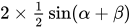
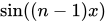
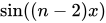
正弦の倍角公式の視覚的な説明。上記の単位辺と角度2θの 二等辺三角形の場合、面積1/2 (底辺 × 高さ) は 2 つ の 。 横向き の は 1/2 sin 2θ です 。 したがって sin 2θ = 2sinθ cosθ と なり ます 。
三重角の公式。[ 20 ]
罪 ( 3 θ ) = 3 罪 θ − 4 罪 3 θ = 4 罪 θ 罪 ( π 3 − θ ) 罪 ( π 3 + θ ) コス ( 3 θ ) = 4 コス 3 θ − 3 コス θ = 4 コス θ コス ( π 3 − θ ) コス ( π 3 + θ ) タン ( 3 θ ) = 3 タン θ − タン 3 θ 1 − 3 タン 2 θ = タン θ タン ( π 3 − θ ) タン ( π 3 + θ ) ベビーベッド ( 3 θ ) = 3 ベビーベッド θ − ベビーベッド 3 θ 1 − 3 ベビーベッド 2 θ 秒 ( 3 θ ) = 秒 3 θ 4 − 3 秒 2 θ csc ( 3 θ ) = csc 3 θ 3 csc 2 θ − 4 {\displaystyle {\begin{aligned}\sin(3\theta )&=3\sin \theta -4\sin ^{3}\theta &&=4\sin \theta \sin \left({\tfrac {\pi }{3}}-\theta \right)\sin \left({\tfrac {\pi }{3}}+\theta \right)\\\cos(3\theta )&=4\cos ^{3}\theta -3\cos \theta &&=4\cos \theta \cos \left({\tfrac {\pi }{3}}-\theta \right)\cos \left({\tfrac {\pi }{3}}+\theta \right)\\\tan(3\theta )&={\frac {3\tan \theta -\tan ^{3}\theta }{1-3\tan ^{2}\theta }}&&=\tan \theta \tan \left({\tfrac {\pi }{3}}-\theta \right)\tan \left({\tfrac {\pi }{3}}+\theta \right)\\\cot(3\theta )&={\frac {3\cot \theta -\cot ^{3}\theta }{1-3\cot ^{2}\theta }}\\\sec(3\theta )&={\frac {\sec ^{3}\theta }{4-3\sec ^{2}\theta }}\\\csc(3\theta )&={\frac {\csc ^{3}\theta }{3\csc ^{2}\theta -4}}\\\end{aligned}}}
複数の角度の公式。[ 22 ]
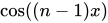
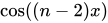
罪 ( n θ ) = ∑ k ∈ O + n ( − 1 ) k − 1 2 ( n k ) コス n − k θ 罪 k θ = 罪 θ ∑ 私 = 0 n + 1 2 ∑ j = 0 私 ( − 1 ) 私 − j ( n 2 私 + 1 ) ( 私 j ) コス n − 2 ( 私 − j ) − 1 θ = 罪 ( θ ) ∑ k = 0 ⌊ n − 1 2 ⌋ ( − 1 ) k ( 2 コス ( θ ) ) n − 2 k − 1 ( n − k − 1 k ) = 2 ( n − 1 ) ∏ k = 0 n − 1 罪 ( k π n + θ ) コス ( n θ ) = ∑ k ∈ E 0 + n ( − 1 ) k 2 ( n k ) コス n − k θ 罪 k θ = ∑ 私 = 0 n 2 ∑ j = 0 私 ( − 1 ) 私 − j ( n 2 私 ) ( 私 j ) コス n − 2 ( 私 − j ) θ = ∑ k = 0 ⌊ n 2 ⌋ ( − 1 ) k ( 2 コス ( θ ) ) n − 2 k ( n − k k ) n 2 n − 2 k コス ( ( 2 n + 1 ) θ ) = ( − 1 ) n 2 2 n ∏ k = 0 2 n コス ( k π 2 n + 1 − θ ) コス ( 2 n θ ) = ( − 1 ) n 2 2 n − 1 ∏ k = 0 2 n − 1 コス ( ( 1 + 2 k ) π 4 n − θ ) タン ( n θ ) = ∑ k ∈ O + n ( − 1 ) k − 1 2 ( n k ) タン k θ ∑ k ∈ E 0 + n ( − 1 ) k 2 ( n k ) タン k θ O + = 正の奇数 E 0 + = 非負の偶数 {\displaystyle {\begin{aligned}\sin(n\theta )&=\sum _{k\in \mathbb {O} ^{+}}^{n}(-1)^{\frac {k-1}{2}}{n \choose k}\cos ^{n-k}\theta \sin ^{k}\theta =\sin \theta \sum _{i=0}^{\frac {n+1}{2}}\sum _{j=0}^{i}(-1)^{i-j}{n \choose 2i+1}{i \choose j}\cos ^{n-2(i-j)-1}\theta \\&=\sin(\theta )\sum _{k=0}^{\left\lfloor {\frac {n-1}{2}}\right\rfloor }(-1)^{k}{\bigl (}2\cos(\theta ){\bigr )}^{n-2k-1}{n-k-1 \choose k}\\&=2^{(n-1)}\prod _{k=0}^{n-1}\sin \left({\frac {k\pi }{n}}+\theta \right)\\\cos(n\theta )&=\sum _{k\in \mathbb {E} _{0}^{+}}^{n}(-1)^{\frac {k}{2}}{n \choose k}\cos ^{n-k}\theta \sin ^{k}\theta =\sum _{i=0}^{\frac {n}{2}}\sum _{j=0}^{i}(-1)^{i-j}{n \choose 2i}{i \choose j}\cos ^{n-2(i-j)}\theta \\&=\sum _{k=0}^{\left\lfloor {\frac {n}{2}}\right\rfloor }(-1)^{k}{(2\cos(\theta ))}^{n-2k}{n-k \choose k}{\frac {n}{2n-2k}}\\\cos {\bigl (}(2n+1)\theta {\bigr )}&=(-1)^{n}2^{2n}\prod _{k=0}^{2n}\cos \left({\frac {k\pi }{2n+1}}-\theta \right)\\\cos(2n\theta )&=(-1)^{n}2^{2n-1}\prod _{k=0}^{2n-1}\cos \left({\frac {(1+2k)\pi }{4n}}-\theta \right)\\\tan(n\theta )&={\frac {\displaystyle \sum _{k\in \mathbb {O} ^{+}}^{n}(-1)^{\frac {k-1}{2}}{n \choose k}\tan ^{k}\theta }{\displaystyle \sum _{k\in \mathbb {E} _{0}^{+}}^{n}(-1)^{\frac {k}{2}}{n \choose k}\tan ^{k}\theta }}\\\mathbb {O} ^{+}&={\text{Positive odd integers}}\\\mathbb {E} _{0}^{+}&={\text{Non-negative even integers}}\\\end{aligned}}}
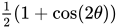
罪 θ 2 = サイン ( 罪 θ 2 ) 1 − コス θ 2 コス θ 2 = サイン ( コス θ 2 ) 1 + コス θ 2 タン θ 2 = 1 − コス θ 罪 θ = 罪 θ 1 + コス θ = csc θ − ベビーベッド θ = タン θ 1 + 秒 θ = サイン ( 罪 θ ) 1 − コス θ 1 + コス θ = − 1 + サイン ( コス θ ) 1 + タン 2 θ タン θ ベビーベッド θ 2 = 1 + コス θ 罪 θ = 罪 θ 1 − コス θ = csc θ + ベビーベッド θ = サイン ( 罪 θ ) 1 + コス θ 1 − コス θ 秒 θ 2 = サイン ( コス θ 2 ) 2 1 + コス θ csc θ 2 = サイン ( 罪 θ 2 ) 2 1 − コス θ {\displaystyle {\begin{aligned}\sin {\frac {\theta }{2}}&=\operatorname {sgn} \left(\sin {\frac {\theta }{2}}\right){\sqrt {\frac {1-\cos \theta }{2}}}\\[3pt]\cos {\frac {\theta }{2}}&=\operatorname {sgn} \left(\cos {\frac {\theta }{2}}\right){\sqrt {\frac {1+\cos \theta }{2}}}\\[3pt]\tan {\frac {\theta }{2}}&={\frac {1-\cos \theta }{\sin \theta }}={\frac {\sin \theta }{1+\cos \theta }}=\csc \theta -\cot \theta ={\frac {\tan \theta }{1+\sec {\theta }}}\\[6mu]&=\operatorname {sgn}(\sin \theta ){\sqrt {\frac {1-\cos \theta }{1+\cos \theta }}}={\frac {-1+\operatorname {sgn}(\cos \theta ){\sqrt {1+\tan ^{2}\theta }}}{\tan \theta }}\\[3pt]\cot {\frac {\theta }{2}}&={\frac {1+\cos \theta }{\sin \theta }}={\frac {\sin \theta }{1-\cos \theta }}=\csc \theta +\cot \theta =\operatorname {sgn}(\sin \theta ){\sqrt {\frac {1+\cos \theta }{1-\cos \theta }}}\\\sec {\frac {\theta }{2}}&=\operatorname {sgn} \left(\cos {\frac {\theta }{2}}\right){\sqrt {\frac {2}{1+\cos \theta }}}\\\csc {\frac {\theta }{2}}&=\operatorname {sgn} \left(\sin {\frac {\theta }{2}}\right){\sqrt {\frac {2}{1-\cos \theta }}}\\\end{aligned}}} [ 25 ] [ 26 ]
また タン η ± θ 2 = 罪 η ± 罪 θ コス η + コス θ タン ( θ 2 + π 4 ) = 秒 θ + タン θ 1 − 罪 θ 1 + 罪 θ = | 1 − タン θ 2 | | 1 + タン θ 2 | {\displaystyle {\begin{aligned}\tan {\frac {\eta \pm \theta }{2}}&={\frac {\sin \eta \pm \sin \theta }{\cos \eta +\cos \theta }}\\[3pt]\tan \left({\frac {\theta }{2}}+{\frac {\pi }{4}}\right)&=\sec \theta +\tan \theta \\[3pt]{\sqrt {\frac {1-\sin \theta }{1+\sin \theta }}}&={\frac {\left|1-\tan {\frac {\theta }{2}}\right|}{\left|1+\tan {\frac {\theta }{2}}\right|}}\end{aligned}}}
テーブル これらは、和と差の公式、または多角公式のいずれかを用いて示すことができる。
正弦と余弦の三角公式が単一の関数のべき乗のみを含むという事実は、コンパスと定規を用いた 角 の三等分作図という幾何学的問題を、三次方程式 を解くという代数的問題と関連付けることを可能にし、それによって、与えられた道具を使って三等分を行うことは一般に不可能であることを証明することができる。
1/3 角の三角関数の恒等式を計算する公式は存在するが、そのためには、3次方程式 4 x 3 − 3 x + d = 0 の零点を求める必要がある。ここで、x は 1/3 角におけるコサイン関数の値、d は 1/3 角におけるコサイン関数の既知の値である。しかし、この方程式の判別式は 正であるため、この方程式には 3 つの実根が存在する (そのうち 1 つだけが 1/3 角のコサインの解である)。これらの解は、 立方根 の中に中間複素数を使用しているため、いずれも実代数式 に還元することはできない。
積和関係と和積関係 二等辺三角形 を用いたプロスタフェレシス計算における和と差から積へのコサイン恒等式の証明積和公式[ 30 ] プロスタフェレシス公式は 、角度加算定理 を使用して右辺を展開することで証明できます。歴史的には、これらのうち最初の4つは、天文学的計算にこれらを使用したヨハネス・ヴェルナー にちなんでヴェルナー公式 として知られていました。[ 31 ] 振幅変調を 、和積公式の応用についてはビート(音響) と位相検出器 を参照してください。
積和関係式 異なる角度の2つの正弦または余弦の積は、それらの角度の和と差の三角関数の和に変換できます。
コス θ コス φ = 1 2 ( コス ( θ − φ ) + コス ( θ + φ ) ) 、 罪 θ 罪 φ = 1 2 ( コス ( θ − φ ) − コス ( θ + φ ) ) 、 罪 θ コス φ = 1 2 ( 罪 ( θ + φ ) + 罪 ( θ − φ ) ) 、 コス θ 罪 φ = 1 2 ( 罪 ( θ + φ ) − 罪 ( θ − φ ) ) 。 {\displaystyle {\begin{aligned}\cos \theta \,\cos \varphi &={\tfrac {1}{2}}{\bigl (}\!\!~\cos(\theta -\varphi )+\cos(\theta +\varphi ){\bigr )},\\[5mu]\sin \theta \,\sin \varphi &={\tfrac {1}{2}}{\bigl (}\!\!~\cos(\theta -\varphi )-\cos(\theta +\varphi ){\bigr )},\\[5mu]\sin \theta \,\cos \varphi &={\tfrac {1}{2}}{\bigl (}\!\!~\sin(\theta +\varphi )+\sin(\theta -\varphi ){\bigr )},\\[5mu]\cos \theta \,\sin \varphi &={\tfrac {1}{2}}{\bigl (}\!\!~\sin(\theta +\varphi )-\sin(\theta -\varphi ){\bigr )}.\end{aligned}}} タン θ タン φ = コス ( θ − φ ) − コス ( θ + φ ) コス ( θ − φ ) + コス ( θ + φ ) 、 タン θ タン φ = 罪 ( θ + φ ) + 罪 ( θ − φ ) 罪 ( θ + φ ) − 罪 ( θ − φ ) 。 {\displaystyle {\begin{aligned}\tan \theta \,\tan \varphi &={\frac {\cos(\theta -\varphi )-\cos(\theta +\varphi )}{\cos(\theta -\varphi )+\cos(\theta +\varphi )}},\\[5mu]{\frac {\tan \theta }{\tan \varphi }}&={\frac {\sin(\theta +\varphi )+\sin(\theta -\varphi )}{\sin(\theta +\varphi )-\sin(\theta -\varphi )}}.\end{aligned}}}
より一般的には、任意の数の正弦または余弦の積に対して、∏ k = 1 n コス θ k = 1 2 n ∑ e ∈ S コス ( e 1 θ 1 + ⋯ + e n θ n ) どこ e = ( e 1 、 … 、 e n ) ∈ S = { 1 、 − 1 } n 、 ∏ k = 1 n 罪 θ k = ( − 1 ) ⌊ n 2 ⌋ 2 n { ∑ e ∈ S コス ( e 1 θ 1 + ⋯ + e n θ n ) ∏ j = 1 n e j もし n さえ 、 ∑ e ∈ S 罪 ( e 1 θ 1 + ⋯ + e n θ n ) ∏ j = 1 n e j もし n 奇妙だ 。 {\displaystyle {\begin{aligned}\prod _{k=1}^{n}\cos \theta _{k}&={\frac {1}{2^{n}}}\sum _{e\in S}\cos(e_{1}\theta _{1}+\cdots +e_{n}\theta _{n})\\[5mu]&{\text{where }}e=(e_{1},\ldots ,e_{n})\in S=\{1,-1\}^{n},\\\prod _{k=1}^{n}\sin \theta _{k}&={\frac {(-1)^{\left\lfloor {\frac {n}{2}}\right\rfloor }}{2^{n}}}{\begin{cases}\displaystyle \sum _{e\in S}\cos(e_{1}\theta _{1}+\cdots +e_{n}\theta _{n})\prod _{j=1}^{n}e_{j}\;{\text{if}}\;n\;{\text{is even}},\\\displaystyle \sum _{e\in S}\sin(e_{1}\theta _{1}+\cdots +e_{n}\theta _{n})\prod _{j=1}^{n}e_{j}\;{\text{if}}\;n\;{\text{is odd}}.\end{cases}}\end{aligned}}}
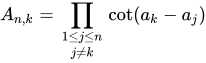
シャルル・エルミートは 次の恒等式を証明した。[ 33 ] 1 1 、 … 、 1 n {\displaystyle a_{1},\ldots ,a_{n}} は複素数 であり、どの2つの数もπ の整数倍だけ異なることはない。
A n 、 k = ∏ 1 ≤ j ≤ n j ≠ k ベビーベッド ( 1 k − 1 j ) {\displaystyle A_{n,k}=\prod _{\begin{smallmatrix}1\leq j\leq n\\j\neq k\end{smallmatrix}}\cot(a_{k}-a_{j})}
(特に、A 1 、 1 、 {\displaystyle A_{1,1},} 空の製品 であるため、 1)となる。
ベビーベッド ( z − 1 1 ) ⋯ ベビーベッド ( z − 1 n ) = コス n π 2 + ∑ k = 1 n A n 、 k ベビーベッド ( z − 1 k ) 。 {\displaystyle \cot(z-a_{1})\cdots \cot(z-a_{n})=\cos {\frac {n\pi }{2}}+\sum _{k=1}^{n}A_{n,k}\cot(z-a_{k}).}
最も単純な非自明な例は、n = 2 の 場合です。
ベビーベッド ( z − 1 1 ) ベビーベッド ( z − 1 2 ) = − 1 + ベビーベッド ( 1 1 − 1 2 ) ベビーベッド ( z − 1 1 ) + ベビーベッド ( 1 2 − 1 1 ) ベビーベッド ( z − 1 2 ) 。 {\displaystyle \cot(z-a_{1})\cot(z-a_{2})=-1+\cot(a_{1}-a_{2})\cot(z-a_{1})+\cot(a_{2}-a_{1})\cot(z-a_{2}).}
三角関数の有限積 互いに素な 整数n とm に対して
∏ k = 1 n ( 2 1 + 2 コス ( 2 π k m n + x ) ) = 2 ( T n ( 1 ) + ( − 1 ) n + m コス ( n x ) ) {\displaystyle \prod _{k=1}^{n}\left(2a+2\cos \left({\frac {2\pi km}{n}}+x\right)\right)=2\left(T_{n}(a)+{(-1)}^{n+m}\cos(nx)\right)}
ここで、T n はチェビシェフ多項式 である。
正弦関数については、以下の関係が成り立つ。
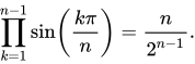
∏ k = 1 n − 1 罪 ( k π n ) = n 2 n − 1 。 {\displaystyle \prod _{k=1}^{n-1}\sin \left({\frac {k\pi }{n}}\right)={\frac {n}{2^{n-1}}}.}
より一般的には、整数n > 0の場合[ 34 ]
罪 ( n x ) = 2 n − 1 ∏ k = 0 n − 1 罪 ( k π n + x ) = 2 n − 1 ∏ k = 1 n 罪 ( k π n − x ) 。 {\displaystyle \sin(nx)=2^{n-1}\prod _{k=0}^{n-1}\sin \left({\frac {k\pi }{n}}+x\right)=2^{n-1}\prod _{k=1}^{n}\sin \left({\frac {k\pi }{n}}-x\right).}
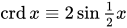
またはコード 機能の観点から記述するクレジット x ≡ 2 罪 1 2 x {\textstyle \operatorname {crd} x\equiv 2\sin {\tfrac {1}{2}}x}
クレジット ( n x ) = ∏ k = 1 n クレジット ( 2 k π n − x ) 。 {\displaystyle \operatorname {crd} (nx)=\prod _{k=1}^{n}\operatorname {crd} \left({\frac {2k\pi }{n}}-x\right).}
これは多項式の因数分解 から得られる。z n − 1 {\textstyle z^{n}-1} 単位根を 参照):任意の複素数z と整数n > 0
z n − 1 = ∏ k = 1 n ( z − exp 2 k 私 π n ) 。 {\displaystyle z^{n}-1=\prod _{k=1}^{n}\left(z-\exp {\frac {2ki\pi }{n}}\right).}
線形結合 目的によっては、周期または周波数が同じだが位相シフトが異なる正弦波の 線形結合 も、周期または周波数は同じだが位相シフトが異なる正弦波であることを知っておくことが重要です。これは正弦波 データのフィッティング に役立ちます。なぜなら、測定または観測されたデータは、以下の同相成分と直交成分の基底の a とb の 未知数と線形関係にあるため、ヤコビアンが 単純になるからです。c {\displaystyle c} φ {\displaystyle \varphi }
正弦と余弦 正弦波と余弦波の線形結合、または調和加算は、位相シフトとスケーリングされた振幅を持つ単一の正弦波に相当します。[ 35 ] [ 36 ]
1 コス x + b 罪 x = c コス ( x + φ ) {\displaystyle a\cos x+b\sin x=c\cos(x+\varphi )}
どこc {\displaystyle c} φ {\displaystyle \varphi }
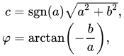
c = サイン ( 1 ) 1 2 + b 2 、 φ = アークタン ( − b 1 ) 、 {\displaystyle {\begin{aligned}c&=\operatorname {sgn}(a){\sqrt {a^{2}+b^{2}}},\\\varphi &=\arctan \left(-{\frac {b}{a}}\right),\end{aligned}}}
とすれば1 ≠ 0. {\displaystyle a\neq 0.}
任意の位相シフト より一般的には、任意の位相シフトに対して、
1 罪 ( x + θ 1 ) + b 罪 ( x + θ b ) = c 罪 ( x + φ ) {\displaystyle a\sin(x+\theta _{a})+b\sin(x+\theta _{b})=c\sin(x+\varphi )}
どこc {\displaystyle c} φ {\displaystyle \varphi }
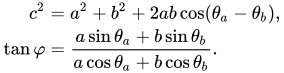
c 2 = 1 2 + b 2 + 2 1 b コス ( θ 1 − θ b ) 、 タン φ = 1 罪 θ 1 + b 罪 θ b 1 コス θ 1 + b コス θ b 。 {\displaystyle {\begin{aligned}c^{2}&=a^{2}+b^{2}+2ab\cos \left(\theta _{a}-\theta _{b}\right),\\\tan \varphi &={\frac {a\sin \theta _{a}+b\sin \theta _{b}}{a\cos \theta _{a}+b\cos \theta _{b}}}.\end{aligned}}}
2つ以上の正弦波 一般的なケースは[ 36 ]
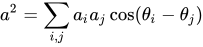
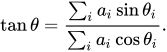
∑ 私 1 私 罪 ( x + θ 私 ) = 1 罪 ( x + θ ) 、 {\displaystyle \sum _{i}a_{i}\sin(x+\theta _{i})=a\sin(x+\theta ),} 1 2 = ∑ 私 、 j 1 私 1 j コス ( θ 私 − θ j ) {\displaystyle a^{2}=\sum _{i,j}a_{i}a_{j}\cos(\theta _{i}-\theta _{j})} タン θ = ∑ 私 1 私 罪 θ 私 ∑ 私 1 私 コス θ 私 。 {\displaystyle \tan \theta ={\frac {\sum _{i}a_{i}\sin \theta _{i}}{\sum _{i}a_{i}\cos \theta _{i}}}.}
ジョセフ・ルイ・ラグランジュ にちなんで名付けられたこれらのアイデンティティは次のとおりです。[ 37 ] [ 38 ] [ 39 ] ∑ k = 0 n 罪 k θ = コス 1 2 θ − コス ( ( n + 1 2 ) θ ) 2 罪 1 2 θ ∑ k = 1 n コス k θ = − 罪 1 2 θ + 罪 ( ( n + 1 2 ) θ ) 2 罪 1 2 θ {\displaystyle {\begin{aligned}\sum _{k=0}^{n}\sin k\theta &={\frac {\cos {\tfrac {1}{2}}\theta -\cos \left(\left(n+{\tfrac {1}{2}}\right)\theta \right)}{2\sin {\tfrac {1}{2}}\theta }}\\[5pt]\sum _{k=1}^{n}\cos k\theta &={\frac {-\sin {\tfrac {1}{2}}\theta +\sin \left(\left(n+{\tfrac {1}{2}}\right)\theta \right)}{2\sin {\tfrac {1}{2}}\theta }}\end{aligned}}} θ ≢ 0 ( モジュール 2 π ) 。 {\displaystyle \theta \not \equiv 0{\pmod {2\pi }}.}
関連する関数として、ディリクレ核 がある。
D n ( θ ) = 1 + 2 ∑ k = 1 n コス k θ = 罪 ( ( n + 1 2 ) θ ) 罪 1 2 θ 。 {\displaystyle D_{n}(\theta )=1+2\sum _{k=1}^{n}\cos k\theta ={\frac {\sin \left(\left(n+{\tfrac {1}{2}}\right)\theta \right)}{\sin {\tfrac {1}{2}}\theta }}.}
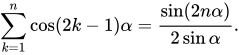
同様の恒等式は[ 40 ]である。
∑ k = 1 n コス ( 2 k − 1 ) α = 罪 ( 2 n α ) 2 罪 α 。 {\displaystyle \sum _{k=1}^{n}\cos(2k-1)\alpha ={\frac {\sin(2n\alpha )}{2\sin \alpha }}.}
証明は次のとおりです。角度の和と差の公式 を使用すると、 罪 ( A + B ) − 罪 ( A − B ) = 2 コス A 罪 B 。 {\displaystyle \sin(A+B)-\sin(A-B)=2\cos A\sin B.}
2 罪 α ∑ k = 1 n コス ( 2 k − 1 ) α = 2 罪 α コス α + 2 罪 α コス 3 α + 2 罪 α コス 5 α + ⋯ + 2 罪 α コス ( 2 n − 1 ) α {\displaystyle 2\sin \alpha \sum _{k=1}^{n}\cos(2k-1)\alpha =2\sin \alpha \cos \alpha +2\sin \alpha \cos 3\alpha +2\sin \alpha \cos 5\alpha +\cdots +2\sin \alpha \cos(2n-1)\alpha }
2 罪 α ∑ k = 1 n コス ( 2 k − 1 ) α = ∑ k = 1 n ( 罪 ( 2 k α ) − 罪 ( 2 ( k − 1 ) α ) ) = ( 罪 2 α − 罪 0 ) + ( 罪 4 α − 罪 2 α ) + ( 罪 6 α − 罪 4 α ) + ⋯ + ( 罪 ( 2 n α ) − 罪 ( 2 ( n − 1 ) α ) ) = 罪 ( 2 n α ) 。 {\displaystyle {\begin{aligned}&2\sin \alpha \sum _{k=1}^{n}\cos(2k-1)\alpha \\&\quad =\sum _{k=1}^{n}(\sin(2k\alpha )-\sin(2(k-1)\alpha ))\\&\quad =(\sin 2\alpha -\sin 0)+(\sin 4\alpha -\sin 2\alpha )+(\sin 6\alpha -\sin 4\alpha )+\cdots +(\sin(2n\alpha )-\sin(2(n-1)\alpha ))\\&\quad =\sin(2n\alpha ).\end{aligned}}}
したがって、この式を割ると2 罪 α {\displaystyle 2\sin \alpha }
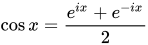
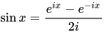
複素指数関数との関係 オイラーの公式によれば、任意の実数 x に対して次のようになる。[ 41 ] e 私 x = コス x + 私 罪 x 、 {\displaystyle e^{ix}=\cos x+i\sin x,} iは 虚数単位 である。xに−x を 代入すると次のようになる。 e − 私 x = コス ( − x ) + 私 罪 ( − x ) = コス x − 私 罪 x 。 {\displaystyle e^{-ix}=\cos(-x)+i\sin(-x)=\cos x-i\sin x.}
これらの 2 つの方程式は、指数関数 に関してコサインとサインを解くために使用できます。具体的には、[ 42 ] [ 43 ] コス x = e 私 x + e − 私 x 2 {\displaystyle \cos x={\frac {e^{ix}+e^{-ix}}{2}}} 罪 x = e 私 x − e − 私 x 2 私 {\displaystyle \sin x={\frac {e^{ix}-e^{-ix}}{2i}}}
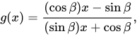
これらの公式は、他の多くの三角関数の恒等式を証明するのに役立ちます。たとえば、 e i ( θ + φ )e iθ e iφ
cos( θ + φ ) + i sin( θ + φ ) = (cos θ + i sin θ ) (cos φ + i sin φ ) = (cos θ cos φ − sin θ sin φ ) + i (cos θ sin φ + sin θ cos φ ) 。
左辺の実数部と右辺の実数部が等しいことは、余弦の角度加算公式である。虚数部が等しいことは、正弦の角度加算公式である。
次の表は、三角関数とその逆関数を指数関数と複素対数 を用いて表したものです。
複素双曲線関数との関係 三角関数は複素 引数を持つ双曲線関数 から導出できます。関係式の公式は以下に示されています[ 45 ] [ 46 ] 罪 x = − 私 シン ( 私 x ) コス x = コッシュ ( 私 x ) タン x = − 私 タン ( 私 x ) ベビーベッド x = 私 布 ( 私 x ) 秒 x = セック ( 私 x ) csc x = 私 csch ( 私 x ) {\displaystyle {\begin{aligned}\sin x&=-i\sinh(ix)\\\cos x&=\cosh(ix)\\\tan x&=-i\tanh(ix)\\\cot x&=i\coth(ix)\\\sec x&=\operatorname {sech} (ix)\\\csc x&=i\operatorname {csch} (ix)\\\end{aligned}}}
シリーズ展開 三角関数を定義するためにべき級数 展開を使用すると、次の恒等式が得られます。[ 47 ]
罪 x = x − x 3 3 ! + x 5 5 ! − x 7 7 ! + ⋯ = ∑ n = 0 ∞ ( − 1 ) n x 2 n + 1 ( 2 n + 1 ) ! コス x = 1 − x 2 2 ! + x 4 4 ! − x 6 6 ! + ⋯ = ∑ n = 0 ∞ ( − 1 ) n x 2 n ( 2 n ) ! {\displaystyle {\begin{aligned}\sin x&=x-{\frac {x^{3}}{3!}}+{\frac {x^{5}}{5!}}-{\frac {x^{7}}{7!}}+\cdots &&=\sum _{n=0}^{\infty }(-1)^{n}{\frac {x^{2n+1}}{(2n+1)!}}\\\cos x&=1-{\frac {x^{2}}{2!}}+{\frac {x^{4}}{4!}}-{\frac {x^{6}}{6!}}+\cdots &&=\sum _{n=0}^{\infty }(-1)^{n}{\frac {x^{2n}}{(2n)!}}\end{aligned}}}
特殊関数 への応用には、三角関数の次の無限積 公式が役立ちます。[ 48 ] [ 49 ]
罪 x = x ∏ n = 1 ∞ ( 1 − x 2 π 2 n 2 ) 、 コス x = ∏ n = 1 ∞ ( 1 − x 2 π 2 ( n − 1 2 ) ) 2 ) 、 シン x = x ∏ n = 1 ∞ ( 1 + x 2 π 2 n 2 ) 、 コッシュ x = ∏ n = 1 ∞ ( 1 + x 2 π 2 ( n − 1 2 ) ) 2 ) 。 {\displaystyle {\begin{aligned}\sin x&=x\prod _{n=1}^{\infty }\left(1-{\frac {x^{2}}{\pi ^{2}n^{2}}}\right),&\cos x&=\prod _{n=1}^{\infty }\left(1-{\frac {x^{2}}{\pi ^{2}\left(n-{\frac {1}{2}}\right)\!{\vphantom {)}}^{2}}}\right),\\[10mu]\sinh x&=x\prod _{n=1}^{\infty }\left(1+{\frac {x^{2}}{\pi ^{2}n^{2}}}\right),&\cosh x&=\prod _{n=1}^{\infty }\left(1+{\frac {x^{2}}{\pi ^{2}\left(n-{\frac {1}{2}}\right)\!{\vphantom {)}}^{2}}}\right).\end{aligned}}}
逆三角関数 以下の恒等式は、三角関数と逆三角関数を合成した結果を示しています。[ 50 ]
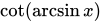
罪 ( arcsin x ) = x コス ( arcsin x ) = 1 − x 2 タン ( arcsin x ) = x 1 − x 2 罪 ( アルコス x ) = 1 − x 2 コス ( アルコス x ) = x タン ( アルコス x ) = 1 − x 2 x 罪 ( アークタン x ) = x 1 + x 2 コス ( アークタン x ) = 1 1 + x 2 タン ( アークタン x ) = x 罪 ( アークスク x ) = 1 x コス ( アークスク x ) = 1 − 1 x 2 タン ( アークスク x ) = 1 x 1 − 1 x 2 罪 ( アークセグ x ) = 1 − 1 x 2 コス ( アークセグ x ) = 1 x タン ( アークセグ x ) = x 1 − 1 x 2 罪 ( アークコット x ) = 1 1 + x 2 コス ( アークコット x ) = x 1 + x 2 タン ( アークコット x ) = 1 x {\displaystyle {\begin{aligned}\sin(\arcsin x)&=x&\cos(\arcsin x)&={\sqrt {1-x^{2}}}&\tan(\arcsin x)&={\frac {x}{\sqrt {1-x^{2}}}}\\\sin(\arccos x)&={\sqrt {1-x^{2}}}&\cos(\arccos x)&=x&\tan(\arccos x)&={\frac {\sqrt {1-x^{2}}}{x}}\\\sin(\arctan x)&={\frac {x}{\sqrt {1+x^{2}}}}&\cos(\arctan x)&={\frac {1}{\sqrt {1+x^{2}}}}&\tan(\arctan x)&=x\\\sin(\operatorname {arccsc} x)&={\frac {1}{x}}&\cos(\operatorname {arccsc} x)&={\sqrt {1-{\frac {1}{x^{2}}}}}&\tan(\operatorname {arccsc} x)&={\frac {1}{x{\sqrt {1-{\frac {1}{x^{2}}}}}}}\\\sin(\operatorname {arcsec} x)&={\sqrt {1-{\frac {1}{x^{2}}}}}&\cos(\operatorname {arcsec} x)&={\frac {1}{x}}&\tan(\operatorname {arcsec} x)&=x{\sqrt {1-{\frac {1}{x^{2}}}}}\\\sin(\operatorname {arccot} x)&={\frac {1}{\sqrt {1+x^{2}}}}&\cos(\operatorname {arccot} x)&={\frac {x}{\sqrt {1+x^{2}}}}&\tan(\operatorname {arccot} x)&={\frac {1}{x}}\\\end{aligned}}}
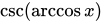
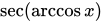
上記の各方程式の両辺の乗法逆数 を取ると、次の式が得られます。csc = 1 罪 、 秒 = 1 コス 、 そして ベビーベッド = 1 タン 。 {\displaystyle \csc ={\frac {1}{\sin }},\;\sec ={\frac {1}{\cos }},{\text{ および }}\cot ={\frac {1}{\tan }}.} ベビーベッド ( arcsin x ) {\displaystyle \cot(\arcsin x)} ベビーベッド ( arcsin x ) = 1 タン ( arcsin x ) = 1 x 1 − x 2 = 1 − x 2 x {\displaystyle \cot(\arcsin x)={\frac {1}{\tan(\arcsin x)}}={\frac {1}{\frac {x}{\sqrt {1-x^{2}}}}}={\frac {\sqrt {1-x^{2}}}{x}}} csc ( アルコス x ) {\displaystyle \csc(\arccos x)} 秒 ( アルコス x ) {\displaystyle \sec(\arccos x)} csc ( アルコス x ) = 1 罪 ( アルコス x ) = 1 1 − x 2 そして 秒 ( アルコス x ) = 1 コス ( アルコス x ) = 1 x 。 {\displaystyle \csc(\arccos x)={\frac {1}{\sin(\arccos x)}}={\frac {1}{\sqrt {1-x^{2}}}}\qquad {\text{ および }}\quad \sec(\arccos x)={\frac {1}{\cos(\arccos x)}}={\frac {1}{x}}.}
以下の恒等式は、反射恒等式 から導かれる。 が成り立つときはいつでも、これらは成り立つ。x 、 r 、 s 、 − x 、 − r 、 {\displaystyle x,r,s,-x,-r,} − s {\displaystyle -s} π 2 = arcsin ( x ) + アルコス ( x ) = アークタン ( r ) + アークコット ( r ) = アークセグ ( s ) + アークスク ( s ) π = アルコス ( x ) + アルコス ( − x ) = アークコット ( r ) + アークコット ( − r ) = アークセグ ( s ) + アークセグ ( − s ) 0 = arcsin ( x ) + arcsin ( − x ) = アークタン ( r ) + アークタン ( − r ) = アークスク ( s ) + アークスク ( − s ) {\displaystyle {\begin{alignedat}{9}{\frac {\pi }{2}}~&=~\arcsin(x)&&+\arccos(x)~&&=~\arctan(r)&&+\operatorname {arccot}(r)~&&=~\operatorname {arcsec}(s)&&+\operatorname {arccsc}(s)\\[0.4ex]\pi ~&=~\arccos(x)&&+\arccos(-x)~&&=~\operatorname {arccot}(r)&&+\operatorname {arccot}(-r)~&&=~\operatorname {arcsec}(s)&&+\operatorname {arcsec}(-s)\\[0.4ex]0~&=~\arcsin(x)&&+\arcsin(-x)~&&=~\arctan(r)&&+\arctan(-r)~&&=~\operatorname {arccsc}(s)&&+\operatorname {arccsc}(-s)\\[1.0ex]\end{alignedat}}}
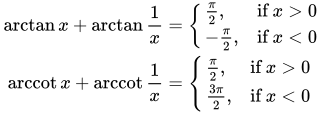
また、[ 51 ] アークタン x + アークタン 1 x = { π 2 、 もし x > 0 − π 2 、 もし x < 0 アークコット x + アークコット 1 x = { π 2 、 もし x > 0 3 π 2 、 もし x < 0 {\displaystyle {\begin{aligned}\arctan x+\arctan {\dfrac {1}{x}}&={\begin{cases}{\frac {\pi }{2}},&{\text{if }}x>0\\-{\frac {\pi }{2}},&{\text{if }}x<0\end{cases}}\\\operatorname {arccot} x+\operatorname {arccot} {\dfrac {1}{x}}&={\begin{cases}{\frac {\pi }{2}},&{\text{if }}x>0\\{\frac {3\pi }{2}},&{\text{if }}x<0\end{cases}}\\\end{aligned}}} アルコス 1 x = アークセグ x そして アークセグ 1 x = アルコス x {\displaystyle \arccos {\frac {1}{x}}=\operatorname {arcsec} x\qquad {\text{ and }}\qquad \operatorname {arcsec} {\frac {1}{x}}=\arccos x} arcsin 1 x = アークスク x そして アークスク 1 x = arcsin x {\displaystyle \arcsin {\frac {1}{x}}=\operatorname {arccsc} x\qquad {\text{ and }}\qquad \operatorname {arccsc} {\frac {1}{x}}=\arcsin x}
逆正接 関数は級数として展開できます。[ 52 ] アークタン ( n x ) = ∑ m = 1 n アークタン x 1 + ( m − 1 ) m x 2 {\displaystyle \arctan(nx)=\sum _{m=1}^{n}\arctan {\frac {x}{1+(m-1)mx^{2}}}}
変数のない恒等式 逆正接 関数に関しては、 [ 51 ] アークタン 1 2 = アークタン 1 3 + アークタン 1 7 {\displaystyle \arctan {\frac {1}{2}}=\arctan {\frac {1}{3}}+\arctan {\frac {1}{7}}}
これはオイラー の逆正接恒等式の特殊なケースである[ 53 ]
アークタン 1 p = アークタン 1 p + q + アークタン q p 2 + p q + 1 。 {\displaystyle \arctan {\frac {1}{p}}=\arctan {\frac {1}{p+q}}+\arctan {\frac {q}{p^{2}+pq+1}}.}
モーリーの法則 として知られる奇妙なアイデンティティ、 コス 20 ∘ ⋅ コス 40 ∘ ⋅ コス 80 ∘ = 1 8 、 {\displaystyle \cos 20^{\circ }\cdot \cos 40^{\circ }\cdot \cos 80^{\circ }={\frac {1}{8}},}
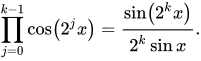
これは、1つの変数を含む恒等式の特殊なケースです。 ∏ j = 0 k − 1 コス ( 2 j x ) = 罪 ( 2 k x ) 2 k 罪 x 。 {\displaystyle \prod _{j=0}^{k-1}\cos \left(2^{j}x\right)={\frac {\sin \left(2^{k}x\right)}{2^{k}\sin x}}.}
同様に、 罪 20 ∘ ⋅ 罪 40 ∘ ⋅ 罪 80 ∘ = 3 8 {\displaystyle \sin 20^{\circ }\cdot \sin 40^{\circ }\cdot \sin 80^{\circ }={\frac {\sqrt {3}}{8}}} x = 20 ∘ {\displaystyle x=20^{\circ }} 罪 x ⋅ 罪 ( 60 ∘ − x ) ⋅ 罪 ( 60 ∘ + x ) = 罪 3 x 4 。 {\displaystyle \sin x\cdot \sin \left(60^{\circ }-x\right)\cdot \sin \left(60^{\circ }+x\right)={\frac {\sin 3x}{4}}.}
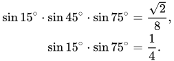
ケースx = 15 ∘ {\displaystyle x=15^{\circ }} 罪 15 ∘ ⋅ 罪 45 ∘ ⋅ 罪 75 ∘ = 2 8 、 罪 15 ∘ ⋅ 罪 75 ∘ = 1 4 。 {\displaystyle {\begin{aligned}\sin 15^{\circ }\cdot \sin 45^{\circ }\cdot \sin 75^{\circ }&={\frac {\sqrt {2}}{8}},\\\sin 15^{\circ }\cdot \sin 75^{\circ }&={\frac {1}{4}}.\end{aligned}}}
ケースx = 10 ∘ {\displaystyle x=10^{\circ }} 罪 10 ∘ ⋅ 罪 50 ∘ ⋅ 罪 70 ∘ = 1 8 。 {\displaystyle \sin 10^{\circ }\cdot \sin 50^{\circ }\cdot \sin 70^{\circ }={\frac {1}{8}}.}
同じコサイン恒等式は コス x ⋅ コス ( 60 ∘ − x ) ⋅ コス ( 60 ∘ + x ) = コス 3 x 4 。 {\displaystyle \cos x\cdot \cos \left(60^{\circ }-x\right)\cdot \cos \left(60^{\circ }+x\right)={\frac {\cos 3x}{4}}.}
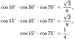
同様に、 コス 10 ∘ ⋅ コス 50 ∘ ⋅ コス 70 ∘ = 3 8 、 コス 15 ∘ ⋅ コス 45 ∘ ⋅ コス 75 ∘ = 2 8 、 コス 15 ∘ ⋅ コス 75 ∘ = 1 4 。 {\displaystyle {\begin{aligned}\cos 10^{\circ }\cdot \cos 50^{\circ }\cdot \cos 70^{\circ }&={\frac {\sqrt {3}}{8}},\\\cos 15^{\circ }\cdot \cos 45^{\circ }\cdot \cos 75^{\circ }&={\frac {\sqrt {2}}{8}},\\\cos 15^{\circ }\cdot \cos 75^{\circ }&={\frac {1}{4}}.\end{aligned}}}
同様に、 タン 50 ∘ ⋅ タン 60 ∘ ⋅ タン 70 ∘ = タン 80 ∘ 、 タン 40 ∘ ⋅ タン 30 ∘ ⋅ タン 20 ∘ = タン 10 ∘ 。 {\displaystyle {\begin{aligned}\tan 50^{\circ }\cdot \tan 60^{\circ }\cdot \tan 70^{\circ }&=\tan 80^{\circ },\\\tan 40^{\circ }\cdot \tan 30^{\circ }\cdot \tan 20^{\circ }&=\tan 10^{\circ }.\end{aligned}}}
以下の内容は、変数を含む恒等式には必ずしも容易に一般化できるものではないかもしれない(ただし、以下の説明を参照のこと)。 コス 24 ∘ + コス 48 ∘ + コス 96 ∘ + コス 168 ∘ = 1 2 。 {\displaystyle \cos 24^{\circ }+\cos 48^{\circ }+\cos 96^{\circ }+\cos 168^{\circ }={\frac {1}{2}}.}
分母に21が含まれるこの恒等式を考えると、度数法はラジアン法よりも優れているとは言えなくなります。 コス 2 π 21 + コス ( 2 ⋅ 2 π 21 ) + コス ( 4 ⋅ 2 π 21 ) + コス ( 5 ⋅ 2 π 21 ) + コス ( 8 ⋅ 2 π 21 ) + コス ( 10 ⋅ 2 π 21 ) = 1 2 。 {\displaystyle \cos {\frac {2\pi }{21}}+\cos \left(2\cdot {\frac {2\pi }{21}}\right)+\cos \left(4\cdot {\frac {2\pi }{21}}\right)+\cos \left(5\cdot {\frac {2\pi }{21}}\right)+\cos \left(8\cdot {\frac {2\pi }{21}}\right)+\cos \left(10\cdot {\frac {2\pi }{21}}\right)={\frac {1}{2}}.}
因数 1、2、4、5、8、10 は、 パターンを明確にし始めるかもしれません。これらは、21/2 より小さい整数で、21 と互いに素である(または共通の素因数を持たない)ものです。 最後 の いくつ か の例は、既約円分多項式に関する基本的な事実の系です。すなわち、コサインはこれらの多項式の零点の実部であり、零点の和は、(上記の最後の例では)21で 評価さ れ たメビウス関数 です。上記の例では零点の半分しか存在しません。この最後のものの前の恒等式は、21 を 15 に置き換えることで同様の方法で得られます。
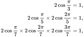
その他のコサイン恒等式には以下が含まれます。[ 54 ] 2 コス π 3 = 1 、 2 コス π 5 × 2 コス 2 π 5 = 1 、 2 コス π 7 × 2 コス 2 π 7 × 2 コス 3 π 7 = 1 、 {\displaystyle {\begin{aligned}2\cos {\frac {\pi }{3}}&=1,\\2\cos {\frac {\pi }{5}}\times 2\cos {\frac {2\pi }{5}}&=1,\\2\cos {\frac {\pi }{7}}\times 2\cos {\frac {2\pi }{7}}\times 2\cos {\frac {3\pi }{7}}&=1,\end{aligned}}} コス π 3 + コス π 5 × コス 2 π 5 + コス π 7 × コス 2 π 7 × コス 3 π 7 + ⋯ = 1. {\displaystyle \cos {\frac {\pi }{3}}+\cos {\frac {\pi }{5}}\times \cos {\frac {2\pi }{5}}+\cos {\frac {\pi }{7}}\times \cos {\frac {2\pi }{7}}\times \cos {\frac {3\pi }{7}}+\dots =1.}
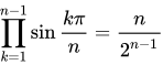
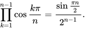
これらの奇妙なアイデンティティの多くは、次のようなより一般的な事実から生じています。[ 55 ] ∏ k = 1 n − 1 罪 k π n = n 2 n − 1 {\displaystyle \prod _{k=1}^{n-1}\sin {\frac {k\pi }{n}}={\frac {n}{2^{n-1}}}} ∏ k = 1 n − 1 コス k π n = 罪 π n 2 2 n − 1 。 {\displaystyle \prod _{k=1}^{n-1}\cos {\frac {k\pi }{n}}={\frac {\sin {\frac {\pi n}{2}}}{2^{n-1}}}.}
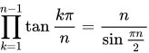
これらを組み合わせると、 ∏ k = 1 n − 1 タン k π n = n 罪 π n 2 {\displaystyle \prod _{k=1}^{n-1}\tan {\frac {k\pi }{n}}={\frac {n}{\sin {\frac {\pi n}{2}}}}}
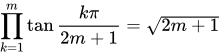
n が奇数の場合(n = 2 m + 1 {\displaystyle n=2m+1} ∏ k = 1 m タン k π 2 m + 1 = 2 m + 1 {\displaystyle \prod _{k=1}^{m}\tan {\frac {k\pi }{2m+1}}={\sqrt {2m+1}}}
バターワース低域通過フィルタ の伝達関数は、多項式と極を用いて表すことができる。周波数をカットオフ周波数 とすることで、次の恒等式が証明できる。 ∏ k = 1 n 罪 ( 2 k − 1 ) π 4 n = ∏ k = 1 n コス ( 2 k − 1 ) π 4 n = 2 2 n {\displaystyle \prod _{k=1}^{n}\sin {\frac {\left(2k-1\right)\pi }{4n}}=\prod _{k=1}^{n}\cos {\frac {\left(2k-1\right)\pi }{4n}}={\frac {\sqrt {2}}{2^{n}}}}
π の計算πを 多数の桁 まで効率的に計算する 方法は、 Machin による以下の変数を用いない恒等式に基づいています。これはMachin式に似た公式 として知られています。 π 4 = 4 アークタン 1 5 − アークタン 1 239 {\displaystyle {\frac {\pi }{4}}=4\arctan {\frac {1}{5}}-\arctan {\frac {1}{239}}} あるいは、レオナルド・オイラー の恒等式を用いる方法もある。 π 4 = 5 アークタン 1 7 + 2 アークタン 3 79 {\displaystyle {\frac {\pi }{4}}=5\arctan {\frac {1}{7}}+2\arctan {\frac {3}{79}}} またはピタゴラス数 を用いる方法: π = アルコス 4 5 + アルコス 5 13 + アルコス 16 65 = arcsin 3 5 + arcsin 12 13 + arcsin 63 65 。 {\displaystyle \pi =\arccos {\frac {4}{5}}+\arccos {\frac {5}{13}}+\arccos {\frac {16}{65}}=\arcsin {\frac {3}{5}}+\arcsin {\frac {12}{13}}+\arcsin {\frac {63}{65}}.}
その他には以下が含まれる:[ 56 ] [ 51 ] π 4 = アークタン 1 2 + アークタン 1 3 、 {\displaystyle {\frac {\pi }{4}}=\arctan {\frac {1}{2}}+\arctan {\frac {1}{3}},} π = アークタン 1 + アークタン 2 + アークタン 3 、 {\displaystyle \pi =\arctan 1+\arctan 2+\arctan 3,} π 4 = 2 アークタン 1 3 + アークタン 1 7 。 {\displaystyle {\frac {\pi }{4}}=2\arctan {\frac {1}{3}}+\arctan {\frac {1}{7}}.}
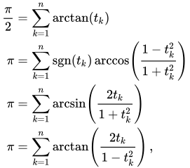
一般に、θ n = Σ n −1 k =1 arctan t k ∈ ( π /4, 3 π /4 )となる数t 1 , ..., t n −1t n = tan( π /2 − θ n ) = cot θ n とします。この最後の式は、接線がt 1 , ..., t n −1 (−1, 1) に t n は 有理数 に なり ます π 2 = ∑ k = 1 n アークタン ( t k ) π = ∑ k = 1 n サイン ( t k ) アルコス ( 1 − t k 2 1 + t k 2 ) π = ∑ k = 1 n arcsin ( 2 t k 1 + t k 2 ) π = ∑ k = 1 n アークタン ( 2 t k 1 − t k 2 ) 、 {\displaystyle {\begin{aligned}{\frac {\pi }{2}}&=\sum _{k=1}^{n}\arctan(t_{k})\\\pi &=\sum _{k=1}^{n}\operatorname {sgn}(t_{k})\arccos \left({\frac {1-t_{k}^{2}}{1+t_{k}^{2}}}\right)\\\pi &=\sum _{k=1}^{n}\arcsin \left({\frac {2t_{k}}{1+t_{k}^{2}}}\right)\\\pi &=\sum _{k=1}^{n}\arctan \left({\frac {2t_{k}}{1-t_{k}^{2}}}\right)\,,\end{aligned}}}
最初の式を除くすべての式で、正接半角の公式を使用しました。最初の 2 つの公式は、t k の 値の 1 つ以上が(−1, 1) の 範囲内にない場合でも機能します。t = p / q が (2 t 、 1 − t 2 、 1 + t 2 )の値は、ピタゴラスの三つ組 (2 pq 、q 2 − p 2 、q 2 + p 2 ) に比例することに注意してください。
例えば、n = 3π 2 = アークタン ( 1 b ) + アークタン ( c d ) + アークタン ( b d − 1 c 1 d + b c ) {\displaystyle {\frac {\pi }{2}}=\arctan \left({\frac {a}{b}}\right)+\arctan \left({\frac {c}{d}}\right)+\arctan \left({\frac {bd-ac}{ad+bc}}\right)} 任意のa 、b 、c 、d > 0
ユークリッドの恒等式 ユークリッドは『 原論 示し た。現代の三角法の言葉で言えば、これは次のようになる。 罪 2 18 ∘ + 罪 2 30 ∘ = 罪 2 36 ∘ 。 {\displaystyle \sin ^{2}18^{\circ }+\sin ^{2}30^{\circ }=\sin ^{2}36^{\circ }.}
プトレマイオスは この命題を用いて、『アルマゲスト』 弦表 におけるいくつかの角度を計算した。
三角関数の合成 これらの恒等式には三角関数の三角関数が含まれています: [ 57 ]
コス ( t 罪 x ) = J 0 ( t ) + 2 ∑ k = 1 ∞ J 2 k ( t ) コス ( 2 k x ) {\displaystyle \cos(t\sin x)=J_{0}(t)+2\sum _{k=1}^{\infty }J_{2k}(t)\cos(2kx)} 罪 ( t 罪 x ) = 2 ∑ k = 0 ∞ J 2 k + 1 ( t ) 罪 ( ( 2 k + 1 ) x ) {\displaystyle \sin(t\sin x)=2\sum _{k=0}^{\infty }J_{2k+1}(t)\sin {\big (}(2k+1)x{\big )}} コス ( t コス x ) = J 0 ( t ) + 2 ∑ k = 1 ∞ ( − 1 ) k J 2 k ( t ) コス ( 2 k x ) {\displaystyle \cos(t\cos x)=J_{0}(t)+2\sum _{k=1}^{\infty }(-1)^{k}J_{2k}(t)\cos(2kx)} 罪 ( t コス x ) = 2 ∑ k = 0 ∞ ( − 1 ) k J 2 k + 1 ( t ) コス ( ( 2 k + 1 ) x ) {\displaystyle \sin(t\cos x)=2\sum _{k=0}^{\infty }(-1)^{k}J_{2k+1}(t)\cos {\big (}(2k+1)x{\big )}} ここで、J i はベッセル関数 である。
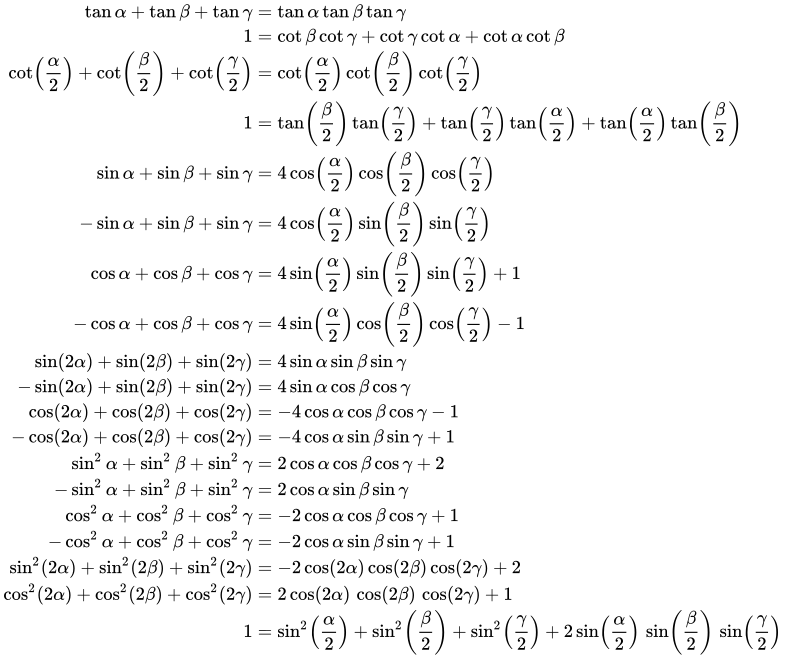
α + β + γ = 180°の場合のさらなる「条件付き」恒等式条件付き三角恒等式 とは、三角関数の引数に関する特定の条件が満たされる場合に成立する三角恒等式のことである。[ 58 ] α + β + γ = 180 ∘ 、 {\displaystyle \alpha +\beta +\gamma =180^{\circ },} [ 59 ] タン α + タン β + タン γ = タン α タン β タン γ 1 = ベビーベッド β ベビーベッド γ + ベビーベッド γ ベビーベッド α + ベビーベッド α ベビーベッド β ベビーベッド ( α 2 ) + ベビーベッド ( β 2 ) + ベビーベッド ( γ 2 ) = ベビーベッド ( α 2 ) ベビーベッド ( β 2 ) ベビーベッド ( γ 2 ) 1 = タン ( β 2 ) タン ( γ 2 ) + タン ( γ 2 ) タン ( α 2 ) + タン ( α 2 ) タン ( β 2 ) 罪 α + 罪 β + 罪 γ = 4 コス ( α 2 ) コス ( β 2 ) コス ( γ 2 ) − 罪 α + 罪 β + 罪 γ = 4 コス ( α 2 ) 罪 ( β 2 ) 罪 ( γ 2 ) コス α + コス β + コス γ = 4 罪 ( α 2 ) 罪 ( β 2 ) 罪 ( γ 2 ) + 1 − コス α + コス β + コス γ = 4 罪 ( α 2 ) コス ( β 2 ) コス ( γ 2 ) − 1 罪 ( 2 α ) + 罪 ( 2 β ) + 罪 ( 2 γ ) = 4 罪 α 罪 β 罪 γ − 罪 ( 2 α ) + 罪 ( 2 β ) + 罪 ( 2 γ ) = 4 罪 α コス β コス γ コス ( 2 α ) + コス ( 2 β ) + コス ( 2 γ ) = − 4 コス α コス β コス γ − 1 − コス ( 2 α ) + コス ( 2 β ) + コス ( 2 γ ) = − 4 コス α 罪 β 罪 γ + 1 罪 2 α + 罪 2 β + 罪 2 γ = 2 コス α コス β コス γ + 2 − 罪 2 α + 罪 2 β + 罪 2 γ = 2 コス α 罪 β 罪 γ コス 2 α + コス 2 β + コス 2 γ = − 2 コス α コス β コス γ + 1 − コス 2 α + コス 2 β + コス 2 γ = − 2 コス α 罪 β 罪 γ + 1 罪 2 ( 2 α ) + 罪 2 ( 2 β ) + 罪 2 ( 2 γ ) = − 2 コス ( 2 α ) コス ( 2 β ) コス ( 2 γ ) + 2 コス 2 ( 2 α ) + コス 2 ( 2 β ) + コス 2 ( 2 γ ) = 2 コス ( 2 α ) コス ( 2 β ) コス ( 2 γ ) + 1 1 = 罪 2 ( α 2 ) + 罪 2 ( β 2 ) + 罪 2 ( γ 2 ) + 2 罪 ( α 2 ) 罪 ( β 2 ) 罪 ( γ 2 ) {\displaystyle {\begin{aligned}\tan \alpha +\tan \beta +\tan \gamma &=\tan \alpha \tan \beta \tan \gamma \\1&=\cot \beta \cot \gamma +\cot \gamma \cot \alpha +\cot \alpha \cot \beta \\\cot \left({\frac {\alpha }{2}}\right)+\cot \left({\frac {\beta }{2}}\right)+\cot \left({\frac {\gamma }{2}}\right)&=\cot \left({\frac {\alpha }{2}}\right)\cot \left({\frac {\beta }{2}}\right)\cot \left({\frac {\gamma }{2}}\right)\\1&=\tan \left({\frac {\beta }{2}}\right)\tan \left({\frac {\gamma }{2}}\right)+\tan \left({\frac {\gamma }{2}}\right)\tan \left({\frac {\alpha }{2}}\right)+\tan \left({\frac {\alpha }{2}}\right)\tan \left({\frac {\beta }{2}}\right)\\\sin \alpha +\sin \beta +\sin \gamma &=4\cos \left({\frac {\alpha }{2}}\right)\cos \left({\frac {\beta }{2}}\right)\cos \left({\frac {\gamma }{2}}\right)\\-\sin \alpha +\sin \beta +\sin \gamma &=4\cos \left({\frac {\alpha }{2}}\right)\sin \left({\frac {\beta }{2}}\right)\sin \left({\frac {\gamma }{2}}\right)\\\cos \alpha +\cos \beta +\cos \gamma &=4\sin \left({\frac {\alpha }{2}}\right)\sin \left({\frac {\beta }{2}}\right)\sin \left({\frac {\gamma }{2}}\right)+1\\-\cos \alpha +\cos \beta +\cos \gamma &=4\sin \left({\frac {\alpha }{2}}\right)\cos \left({\frac {\beta }{2}}\right)\cos \left({\frac {\gamma }{2}}\right)-1\\\sin(2\alpha )+\sin(2\beta )+\sin(2\gamma )&=4\sin \alpha \sin \beta \sin \gamma \\-\sin(2\alpha )+\sin(2\beta )+\sin(2\gamma )&=4\sin \alpha \cos \beta \cos \gamma \\\cos(2\alpha )+\cos(2\beta )+\cos(2\gamma )&=-4\cos \alpha \cos \beta \cos \gamma -1\\-\cos(2\alpha )+\cos(2\beta )+\cos(2\gamma )&=-4\cos \alpha \sin \beta \sin \gamma +1\\\sin ^{2}\alpha +\sin ^{2}\beta +\sin ^{2}\gamma &=2\cos \alpha \cos \beta \cos \gamma +2\\-\sin ^{2}\alpha +\sin ^{2}\beta +\sin ^{2}\gamma &=2\cos \alpha \sin \beta \sin \gamma \\\cos ^{2}\alpha +\cos ^{2}\beta +\cos ^{2}\gamma &=-2\cos \alpha \cos \beta \cos \gamma +1\\-\cos ^{2}\alpha +\cos ^{2}\beta +\cos ^{2}\gamma &=-2\cos \alpha \sin \beta \sin \gamma +1\\\sin ^{2}(2\alpha )+\sin ^{2}(2\beta )+\sin ^{2}(2\gamma )&=-2\cos(2\alpha )\cos(2\beta )\cos(2\gamma )+2\\\cos ^{2}(2\alpha )+\cos ^{2}(2\beta )+\cos ^{2}(2\gamma )&=2\cos(2\alpha )\,\cos(2\beta )\,\cos(2\gamma )+1\\1&=\sin ^{2}\left({\frac {\alpha }{2}}\right)+\sin ^{2}\left({\frac {\beta }{2}}\right)+\sin ^{2}\left({\frac {\gamma }{2}}\right)+2\sin \left({\frac {\alpha }{2}}\right)\,\sin \left({\frac {\beta }{2}}\right)\,\sin \left({\frac {\gamma }{2}}\right)\end{aligned}}}
その他
ディリクレ核 ディリクレ核 D n ( x )1 + 2 コス x + 2 コス ( 2 x ) + 2 コス ( 3 x ) + ⋯ + 2 コス ( n x ) = 罪 ( ( n + 1 2 ) x ) 罪 ( 1 2 x ) 。 {\displaystyle 1+2\cos x+2\cos(2x)+2\cos(3x)+\cdots +2\cos(nx)={\frac {\sin \left(\left(n+{\frac {1}{2}}\right)x\right)}{\sin \left({\frac {1}{2}}x\right)}}.}
周期の任意の 積分可能な関数 の畳み込み2 π {\displaystyle 2\pi } n {\displaystyle n} 測度 または一般化関数 にも当てはまります。
コス θ 2 ⋅ コス θ 4 ⋅ コス θ 8 ⋯ = ∏ n = 1 ∞ コス θ 2 n = 罪 θ θ = シン θ 。 {\displaystyle \cos {\frac {\theta }{2}}\cdot \cos {\frac {\theta }{4}}\cdot \cos {\frac {\theta }{8}}\cdots =\prod _{n=1}^{\infty }\cos {\frac {\theta }{2^{n}}}={\frac {\sin \theta }{\theta }}=\operatorname {sinc} \theta .}
医療画像処理で使用される正弦関数 これは、医用画像処理 の研究の副産物として発見された身元である。[ 61 ]
させて私 = − 1 {\displaystyle i={\sqrt {-1}}} ∘ を 微分作用素の合成を表すものとする。すると、任意の 奇数の正の整数n に対して、
∑ k = 0 n ( n k ) ( d d x − 罪 x ) ∘ ( d d x − 罪 x + 私 ) ∘ ⋯ ⋯ ∘ ( d d x − 罪 x + ( k − 1 ) 私 ) ( 罪 x ) n − k = 0. {\displaystyle {\begin{aligned}\sum _{k=0}^{n}{\binom {n}{k}}\left({\frac {d}{dx}}-\sin x\right)&\circ \left({\frac {d}{dx}}-\sin x+i\right)\circ \cdots \\\cdots &\circ \left({\frac {d}{dx}}-\sin x+(k-1)i\right)(\sin x)^{n-k}=0.\end{aligned}}} (k = 0 の場合、合成される微分演算子の数は 0 なので、上記の和における対応する項は(sin x ) n
参考文献 ↑ アブラモウィッツ、ミルトン ;ステガン、アイリーン・アン 編(1983年)[1964年6月]。「第4章、式4.3.45」。『数式、グラフ、数表付き数学関数ハンドブック 55巻(第10版(1972年12月)の修正を加えた第9版再版 )。ワシントンDC;ニューヨーク:米国商務省国立標準局;ドーバー出版。73 ページ。ISBN 978-0-486-61272-0 . LCCN 64-60036 . MR 0167642 . LCCN 65-12253 . ↑ セルビー 1970 、p.188 ↑ アブラモヴィッツとステガン、p. 72、4.3.13–15 ↑ アブラモヴィッツとステガン、p. 72、4.3.7–9 ↑ アブラモヴィッツとステガン、p. 72、4.3.16 1 2 3 4 ワイスタイン、エリック W. 「三角関数の加算公式」 。 マスワールド 。 ↑ アブラモヴィッツとステガン、p. 72、4.3.17 ↑ アブラモヴィッツとステガン、p. 72、4.3.18 1 2 「角度の和と差の恒等式」 。www.milefoot.com 。 2019年10月12日 取得 。 ↑ アブラモヴィッツとステガン、p. 72、4.3.19 ↑ アブラモヴィッツとステガン、p. 80、4.4.32 ↑ アブラモヴィッツとステガン、p. 80、4.4.33 ↑ アブラモヴィッツとステガン、p. 80、4.4.34 ↑ ブロンスタイン、マヌエル (1989)。「実数初等関数の簡略化」。ゴネット、GH (編) 『 ACM-SIGSAM 1989 国際シンポジウム シンボリック・代数計算 ISSAC '89 議事録』 ( 米国 オレゴン 州ポートランド、1989年7 月 )。ニューヨーク: ACM。pp . 207–211。doi : 10.1145/74540.74566。ISBN 0-89791-325-6 。↑ マイケル・ハーディ (2016). 「無限和の接線と割線について」『アメリカ数学月報』 第123巻、第7号、701–703頁。https ://doi.org/10.4169/amer.math.monthly.123.7.701 ↑ Hardy, Michael (2025). "Invariance of the Cauchy Family Under Linear Fractional Transformations". The American Mathematical Monthly . 132 (5): 453–455 . doi : 10.1080/00029890.2025.2459048 . ↑ Knight, FB ( 1976 ). 「コーシー型の特徴付け」 アメリカ数学会紀要 1976 : 130–135 . ↑ Hardy, Michael (2016). "無限和の接線と割線について" . American Mathematical Monthly . 123 (7): 701– 703. doi : 10.4169/amer.math.monthly.123.7.701 . 1 2 「正弦、余弦、プトレマイオスの定理」 。 1 2 セルビー 1970、190 ページ ↑ 引用エラー: 指定された名前の参照A&Sが呼び出されましたが、定義されていません (ヘルプ ページを参照してください)。 ↑ Weisstein, Eric W. 「多角公式」 . mathworld.wolfram.com . 2022年2月6日 取得 。 ↑ ウォード、ケン。 「複数の角度の再帰式」 。 ケン・ウォードの数学ページ 。 1 2 ワイスタイン、エリック W. 「多角式」 。 マスワールド 。 1 2 アブラモウィッツ、ミルトン ; ステガン、アイリーン・アン 編(1983年)[1964年6月]。 「第4章、式4.3.20-22」 。 『数式、グラフ、数表付き数学関数ハンドブック 』 。応用数学シリーズ。第 55巻(第10版(1972年12月)の修正を加えた第9版再版 )。ワシントンDC;ニューヨーク:米国商務省国立標準局;ドーバー出版。72 ページ 。ISBN 978-0-486-61272-0 . LCCN 64-60036 . MR 0167642 . LCCN 65-12253 . 1 2 ワイスタイン、エリック W. 「半角公式」 。 マスワールド 。 ↑ アブラモヴィッツとステガン、p. 72、4.3.24–26 ↑ Weisstein, Eric W. 「倍角公式」 . MathWorld . ↑ アブラモヴィッツとステガン、p. 72、4.3.27–28 ↑ アブラモヴィッツとステガン、p. 72、4.3.31–33 ↑ イヴス、ハワード(1990)。 数学史入門 (第6 版)。フィラデルフィア:サウンダーズ・カレッジ出版。309 ページ 。ISBN 0-03-029558-0 OCLC 20842510 1 2 アブラモヴィッツとステガン、p. 72、4.3.34–39 ↑ Johnson, Warren P. (2010年4月). "エルミート式による三角関数の恒等式". American Mathematical Monthly . 117 (4): 311–327 . doi : 10.4169/000298910x480784 . S2CID 29690311 . ↑ 「製品のアイデンティティを多角的に捉える 」 ↑ アポストル、TM (1967) 微積分。第2版。ニューヨーク、NY、ワイリー。334-335頁。 1 2 Weisstein, Eric W. 「調和加法定理」 . MathWorld . ↑ Ortiz Muñiz, Eddie (1953 年 2 月). 「ラグランジュの三角恒等式を用いた静電気学および電磁気学における様々な公式の導出方法」 American Journal of Physics . 21 (2): 140. Bibcode : 1953AmJPh..21..140M . doi : 10.1119/1.1933371 . ↑ Agarwal, Ravi P.; O'Regan, Donal (2008). Ordinary and Partial Differential Equations: With Special Functions, Fourier Series, and Boundary Value Problems (illustrated ed.). Springer Science & Business Media. p. 185. ISBN 978-0-387-79146-3 。↑ ジェフリー、アラン;ダイ、フイフイ(2008)。「セクション 2.4.1.6」。 数学公式と積分ハンドブック (第4 版)。アカデミックプレス 。ISBN 978-0-12-374288-9 。↑ Fay, Temple H.; Kloppers, P. Hendrik (2001). "ギブスの現象" . International Journal of Mathematical Education in Science and Technology . 32 (1): 73– 89. doi : 10.1080/00207390117151 . ↑ アブラモヴィッツとステガン、p. 74、4.3.47 ↑ アブラモヴィッツとステガン、p. 71、4.3.2 ↑ アブラモヴィッツとステガン、p. 71、4.3.1 ↑ アブラモヴィッツとステガン、p. 80、4.4.26–31 ↑ ホーキンス、フェイス・メアリー、ホーキンス、JQ(1969年3月1日)。 複素数 と初等複素関数 。ロンドン:マクドナルド・テクニカル&サイエンティフィック・ロンドン(1968年出版)。p. 122。ISBN 978-0356025056 。↑ Markushevich, AI (1966). The Remarkable Sine Function . New York: American Elsevier Publishing Company, Inc. pp. 35–37 , 81. ISBN 978-1483256313 。↑ アブラモヴィッツとステガン、p. 74、4.3.65–66 ↑ アブラモヴィッツとステガン、p. 75、4.3.89–90 ↑ アブラモヴィッツとステガン、p. 85、4.5.68–69 ↑ Abramowitz & Stegun 1972 、p. 73、4.3.45 1 2 3 Wu, Rex H.「言葉のない証明:オイラーの逆正接恒等式」 Mathematics Magazine 77(3)、2004年6月、p. 189。 ↑ SM Abrarov; RK Jagpal; R. Siddiqui; BM Quine (2021), "Algorithmic determination of a large integer in the two-term Machin-like formula for π ", Mathematics , 9 (17), 2162, arXiv : 2107.01027 , doi : 10.3390/math9172162 ↑ オイラー、レオンハルト (1737)。 「De Variis Modis Circvli Qvadratorvm: Numeris Proximae Expremendi」 。 p. 231 . 2026 年 3 月 18 日 に取得 。 ↑ ハンブル、スティーブ(2004年11月)。「おばあちゃん の アイデンティティ 」 。Mathematical Gazette。88 : 524–525。doi : 10.1017 / s0025557200176223。S2CID 125105552 。 ↑ Weisstein, Eric W. "Sine" . MathWorld . ↑ ハリス、エドワード M.「逆正接の和」、ロジャー B. ネルソン編『言葉のない証明』 (1993 年、アメリカ数学協会)、39 ページ。 ↑ ミルトン・アブラモウィッツ、アイリーン・ステガン著『数式、グラフ、数表付き数学関数ハンドブック』 、ドーバー出版 、ニューヨーク、1972年、数式9.1.42~9.1.45↑ えー。 KC Joshi、クリシュナの IIT MATHEMATIKA 。クリシュナ・プラカシャン・メディア。メーラト、インド。 636ページ。 ↑ Cagnoli、Antonio (1808)、 Trigonométrie rectiline et sphérique 、p. 27. ↑ アブラモヴィッツとステガン、p. 72、4.3.23 ↑ Kuchment, Peter; Lvin, Sergey (2013 年 8 月). "Identities for sin x that Came from Medical Imaging". American Mathematical Monthly . 120 (7): 609– 621. arXiv : 1110.6109 . doi : 10.4169/amer.math.monthly.120.07.609 . S2CID 17478608 .
外部リンク 3°と5 + 5 / 8 ° ) 










![{\displaystyle {\begin{aligned}\operatorname {sgn} (\sin \theta )=\operatorname {sgn} (\csc \theta )&={\begin{cases}+1&{\text{if}}\ \ 0<\theta <\pi \\-1&{\text{if}}\ \ {-\pi }<\theta <0\\0&{\text{if}}\ \ \theta \in \{0,\pi \}\end{cases}}\\[5mu]\operatorname {sgn} (\cos \theta )=\operatorname {sgn} (\sec \theta )&={\begin{cases}+1&{\text{if}}\ \ {-{\tfrac {\pi }{2}}}<\theta <{\tfrac {\pi }{2}}\\-1&{\text{if}}\ \ {-\pi }<\theta <-{\tfrac {\pi }{2}}\ \ {\text{or}}\ \ {\tfrac {\pi }{2}}<\theta <\pi \\0&{\text{if}}\ \ \theta \in {\bigl \{}{-{\tfrac {\pi }{2}}},{\tfrac {\pi }{2}}{\bigr \}}\end{cases}}\\[5mu]\operatorname {sgn} (\tan \theta )=\operatorname {sgn} (\cot \theta )&={\begin{cases}+1&{\text{if}}\ \ {-\pi }<\theta <-{\tfrac {\pi }{2}}\ \ {\text{or}}\ \ 0<\theta <{\tfrac {\pi }{2}}\\-1&{\text{if}}\ \ {-{\tfrac {\pi }{2}}}<\theta <0\ \ {\text{or}}\ \ {\tfrac {\pi }{2}}<\theta <\pi \\0&{\text{if}}\ \ \theta \in {\bigl \{}{-{\tfrac {\pi }{2}}},0,{\tfrac {\pi }{2}},\pi {\bigr \}}\end{cases}}\end{aligned}}}](https://wikimedia.org/api/rest_v1/media/math/render/svg/3885aee3a70a73da0b369ad2f21a8122f4e78587)

![{\displaystyle ({-\pi },\pi ],}](https://wikimedia.org/api/rest_v1/media/math/render/svg/122328145a5f3a4162d21b4fbb5f4d1149932d2b)














![{\displaystyle {\begin{aligned}e_{0}&=1\\[6pt]e_{1}&=\sum _{i}x_{i}&&=\sum _{i}\tan \theta _{i}\\[6pt]e_{2}&=\sum _{i<j}x_{i}x_{j}&&=\sum _{i<j}\tan \theta _{i}\tan \theta _{j}\\[6pt]e_{3}&=\sum _{i<j<k}x_{i}x_{j}x_{k}&&=\sum _{i<j<k}\tan \theta _{i}\tan \theta _{j}\tan \theta _{k}\\&\ \ \vdots &&\ \ \vdots \end{aligned}}}](https://wikimedia.org/api/rest_v1/media/math/render/svg/cb1927ae2be96f5156e18813a20486fdb0ff72f1)

![{\displaystyle {\begin{aligned}\tan {\Bigl (}\sum _{i}\theta _{i}{\Bigr )}&={\frac {{\sin }{\bigl (}\sum _{i}\theta _{i}{\bigr )}/\prod _{i}\cos \theta _{i}}{{\cos }{\bigl (}\sum _{i}\theta _{i}{\bigr )}/\prod _{i}\cos \theta _{i}}}\\[10pt]&={\frac {\displaystyle \sum _{{\text{odd}}\ k\geq 1}(-1)^{\frac {k-1}{2}}\sum _{\begin{smallmatrix}A\subseteq \{1,2,3,\dots \}\\\left|A\right|=k\end{smallmatrix}}\prod _{i\in A}\tan \theta _{i}}{\displaystyle \sum _{{\text{even}}\ k\geq 0}~(-1)^{\frac {k}{2}}~~\sum _{\begin{smallmatrix}A\subseteq \{1,2,3,\dots \}\\\left|A\right|=k\end{smallmatrix}}\prod _{i\in A}\tan \theta _{i}}}={\frac {e_{1}-e_{3}+e_{5}-\cdots }{e_{0}-e_{2}+e_{4}-\cdots }}\\[10pt]\cot {\Bigl (}\sum _{i}\theta _{i}{\Bigr )}&={\frac {e_{0}-e_{2}+e_{4}-\cdots }{e_{1}-e_{3}+e_{5}-\cdots }}\end{aligned}}}](https://wikimedia.org/api/rest_v1/media/math/render/svg/55ff3a24e1e073c731c170651eca41efdad72212)
![{\displaystyle {\begin{aligned}\tan(\theta _{1}+\theta _{2})&={\frac {e_{1}}{e_{0}-e_{2}}}={\frac {x_{1}+x_{2}}{1\ -\ x_{1}x_{2}}}={\frac {\tan \theta _{1}+\tan \theta _{2}}{1\ -\ \tan \theta _{1}\tan \theta _{2}}},\\[8pt]\tan(\theta _{1}+\theta _{2}+\theta _{3})&={\frac {e_{1}-e_{3}}{e_{0}-e_{2}}}={\frac {(x_{1}+x_{2}+x_{3})\ -\ (x_{1}x_{2}x_{3})}{1\ -\ (x_{1}x_{2}+x_{1}x_{3}+x_{2}x_{3})}},\\[8pt]\tan(\theta _{1}+\theta _{2}+\theta _{3}+\theta _{4})&={\frac {e_{1}-e_{3}}{e_{0}-e_{2}+e_{4}}}\\[8pt]&={\frac {(x_{1}+x_{2}+x_{3}+x_{4})\ -\ (x_{1}x_{2}x_{3}+x_{1}x_{2}x_{4}+x_{1}x_{3}x_{4}+x_{2}x_{3}x_{4})}{1\ -\ (x_{1}x_{2}+x_{1}x_{3}+x_{1}x_{4}+x_{2}x_{3}+x_{2}x_{4}+x_{3}x_{4})\ +\ (x_{1}x_{2}x_{3}x_{4})}},\end{aligned}}}](https://wikimedia.org/api/rest_v1/media/math/render/svg/4c9196b8ab5e0aef6cf7d7fec7d7546f2a6e7d2f)


![{\displaystyle {\begin{aligned}{\sec }{\Bigl (}\sum _{i}\theta _{i}{\Bigr )}&={\frac {\prod _{i}\sec \theta _{i}}{e_{0}-e_{2}+e_{4}-\cdots }}\\[8pt]{\csc }{\Bigl (}\sum _{i}\theta _{i}{\Bigr )}&={\frac {\prod _{i}\sec \theta _{i}}{e_{1}-e_{3}+e_{5}-\cdots }}\end{aligned}}}](https://wikimedia.org/api/rest_v1/media/math/render/svg/b24f2b169fbe11608507c63f5bb728e03b2b4957)


![{\displaystyle {\begin{aligned}\sec(\alpha +\beta +\gamma )&={\frac {\sec \alpha \sec \beta \sec \gamma }{1-\tan \alpha \tan \beta -\tan \alpha \tan \gamma -\tan \beta \tan \gamma }}\\[8pt]\csc(\alpha +\beta +\gamma )&={\frac {\sec \alpha \sec \beta \sec \gamma }{\tan \alpha +\tan \beta +\tan \gamma -\tan \alpha \tan \beta \tan \gamma }}.\end{aligned}}}](https://wikimedia.org/api/rest_v1/media/math/render/svg/e082e69aab7a9c782f590f3a93262ba3101899b7)















![{\displaystyle {\begin{aligned}\sin {\frac {\theta }{2}}&=\operatorname {sgn} \left(\sin {\frac {\theta }{2}}\right){\sqrt {\frac {1-\cos \theta }{2}}}\\[3pt]\cos {\frac {\theta }{2}}&=\operatorname {sgn} \left(\cos {\frac {\theta }{2}}\right){\sqrt {\frac {1+\cos \theta }{2}}}\\[3pt]\tan {\frac {\theta }{2}}&={\frac {1-\cos \theta }{\sin \theta }}={\frac {\sin \theta }{1+\cos \theta }}=\csc \theta -\cot \theta ={\frac {\tan \theta }{1+\sec {\theta }}}\\[6mu]&=\operatorname {sgn} (\sin \theta ){\sqrt {\frac {1-\cos \theta }{1+\cos \theta }}}={\frac {-1+\operatorname {sgn} (\cos \theta ){\sqrt {1+\tan ^{2}\theta }}}{\tan \theta }}\\[3pt]\cot {\frac {\theta }{2}}&={\frac {1+\cos \theta }{\sin \theta }}={\frac {\sin \theta }{1-\cos \theta }}=\csc \theta +\cot \theta =\operatorname {sgn} (\sin \theta ){\sqrt {\frac {1+\cos \theta }{1-\cos \theta }}}\\\sec {\frac {\theta }{2}}&=\operatorname {sgn} \left(\cos {\frac {\theta }{2}}\right){\sqrt {\frac {2}{1+\cos \theta }}}\\\csc {\frac {\theta }{2}}&=\operatorname {sgn} \left(\sin {\frac {\theta }{2}}\right){\sqrt {\frac {2}{1-\cos \theta }}}\\\end{aligned}}}](https://wikimedia.org/api/rest_v1/media/math/render/svg/d53d104c73c4b28f1dd7bfa5d2b0c7207c68cd87)
![{\displaystyle {\begin{aligned}\tan {\frac {\eta \pm \theta }{2}}&={\frac {\sin \eta \pm \sin \theta }{\cos \eta +\cos \theta }}\\[3pt]\tan \left({\frac {\theta }{2}}+{\frac {\pi }{4}}\right)&=\sec \theta +\tan \theta \\[3pt]{\sqrt {\frac {1-\sin \theta }{1+\sin \theta }}}&={\frac {\left|1-\tan {\frac {\theta }{2}}\right|}{\left|1+\tan {\frac {\theta }{2}}\right|}}\end{aligned}}}](https://wikimedia.org/api/rest_v1/media/math/render/svg/639270245e163f1afa8682ac8aa12086db43dce1)

















![{\displaystyle {\begin{aligned}\cos \theta \,\cos \varphi &={\tfrac {1}{2}}{\bigl (}\!\!~\cos(\theta -\varphi )+\cos(\theta +\varphi ){\bigr )},\\[5mu]\sin \theta \,\sin \varphi &={\tfrac {1}{2}}{\bigl (}\!\!~\cos(\theta -\varphi )-\cos(\theta +\varphi ){\bigr )},\\[5mu]\sin \theta \,\cos \varphi &={\tfrac {1}{2}}{\bigl (}\!\!~\sin(\theta +\varphi )+\sin(\theta -\varphi ){\bigr )},\\[5mu]\cos \theta \,\sin \varphi &={\tfrac {1}{2}}{\bigl (}\!\!~\sin(\theta +\varphi )-\sin(\theta -\varphi ){\bigr )}.\end{aligned}}}](https://wikimedia.org/api/rest_v1/media/math/render/svg/dcd715f4b6380798a701537d9c067f28cc371efa)
![{\displaystyle {\begin{aligned}\tan \theta \,\tan \varphi &={\frac {\cos(\theta -\varphi )-\cos(\theta +\varphi )}{\cos(\theta -\varphi )+\cos(\theta +\varphi )}},\\[5mu]{\frac {\tan \theta }{\tan \varphi }}&={\frac {\sin(\theta +\varphi )+\sin(\theta -\varphi )}{\sin(\theta +\varphi )-\sin(\theta -\varphi )}}.\end{aligned}}}](https://wikimedia.org/api/rest_v1/media/math/render/svg/69a3a5dee2394b1ed85551729df20f0abd6770b7)
![{\displaystyle {\begin{aligned}\prod _{k=1}^{n}\cos \theta _{k}&={\frac {1}{2^{n}}}\sum _{e\in S}\cos(e_{1}\theta _{1}+\cdots +e_{n}\theta _{n})\\[5mu]&{\text{ただし}}e=(e_{1},\ldots ,e_{n})\in S=\{1,-1\}^{n},\\\prod _{k=1}^{n}\sin \theta _{k}&={\frac {(-1)^{\left\lfloor {\frac {n}{2}}\right\rfloor }}{2^{n}}}{\begin{cases}\displaystyle \sum _{e\in \end{cases}}\end{aligned}}}](https://wikimedia.org/api/rest_v1/media/math/render/svg/106ce6115e77f036a95a2096bc66b01927e5dff9)


![{\displaystyle {\begin{aligned}\sin \theta +\sin \varphi &=2\sin {\tfrac {1}{2}}(\theta +\varphi )\,\cos {\tfrac {1}{2}}(\theta -\varphi ),\\[5mu]\sin \theta -\sin \varphi &=2\cos {\tfrac {1}{2}}(\theta +\varphi )\,\sin {\tfrac {1}{2}}(\theta -\varphi ),\\[5mu]\cos \theta +\cos \varphi &=2\cos {\tfrac {1}{2}}(\theta +\varphi )\,\cos {\tfrac {1}{2}}(\theta -\varphi ),\\[5mu]\cos \theta -\cos \varphi &=-2\sin {\tfrac {1}{2}}(\theta +\varphi )\,\sin {\tfrac {1}{2}}(\theta -\varphi ).\end{aligned}}}](https://wikimedia.org/api/rest_v1/media/math/render/svg/3676cbeab42be735d5fb198d843eeec23ee9b763)













![{\displaystyle {\begin{aligned}\sum _{k=0}^{n}\sin k\theta &={\frac {\cos {\tfrac {1}{2}}\theta -\cos \left(\left(n+{\tfrac {1}{2}}\right)\theta \right)}{2\sin {\tfrac {1}{2}}\theta }}\\[5pt]\sum _{k=1}^{n}\cos k\theta &={\frac {-\sin {\tfrac {1}{2}}\theta +\sin \left(\left(n+{\tfrac {1}{2}}\right)\theta \right)}{2\sin {\tfrac {1}{2}}\theta }}\end{aligned}}}](https://wikimedia.org/api/rest_v1/media/math/render/svg/4679d7bb8112018d06e7d3a849bbe4ce024ff148)












![{\displaystyle {\begin{aligned}\sin x&=x\prod _{n=1}^{\infty }\left(1-{\frac {x^{2}}{\pi ^{2}n^{2}}}\right),&\cos x&=\prod _{n=1}^{\infty }\left(1-{\frac {x^{2}}{\pi ^{2}\left(n-{\frac {1}{2}}\right)\!{\vphantom {)}}^{2}}}\right),\\[10mu]\sinh x&=x\prod _{n=1}^{\infty }\left(1+{\frac {x^{2}}{\pi ^{2}n^{2}}}\right),&\cosh x&=\prod _{n=1}^{\infty }\left(1+{\frac {x^{2}}{\pi ^{2}\left(n-{\frac {1}{2}}\right)\!{\vphantom {)}}^{2}}}\right).\end{aligned}}}](https://wikimedia.org/api/rest_v1/media/math/render/svg/6d43e1176a38b1e6b653837eb782ae79735783ac)






![{\displaystyle {\begin{alignedat}{9}{\frac {\pi }{2}}~&=~\arcsin(x)&&+\arccos(x)~&&=~\arctan(r)&&+\operatorname {arccot} (r)~&&=~\operatorname {arcsec} (s)&&+\operatorname {arccsc} (s)\\[0.4ex]\pi ~&=~\arccos(x)&&+\arccos(-x)~&&=~\operatorname {arccot} (r)&&+\operatorname {arccot} (-r)~&&=~\operatorname {arcsec} (s)&&+\operatorname {arcsec} (-s)\\[0.4ex]0~&=~\arcsin(x)&&+\arcsin(-x)~&&=~\arctan(r)&&+\arctan(-r)~&&=~\operatorname {arccsc} (s)&&+\operatorname {arccsc} (-s)\\[1.0ex]\end{alignedat}}}](https://wikimedia.org/api/rest_v1/media/math/render/svg/839db041f421b4af5890106450e2b4d3e9e183d4)