Representations of finite groups, particularly on vector spaces
群 の 表現 理論 は、与えられた構造に対して群がどのように作用するかを調べる数学の一部です。
ここでは特に ベクトル空間 上の 群の演算に焦点を当てます。ただし、他の群や 集合 に作用する群も 考慮されます。詳細については、置換表現のセクションを参照してください。
いくつかの顕著な例外を除き、本稿では有限群のみを考察する。また、 特性 ゼロの 体上のベクトル空間に限定する。特性ゼロの 代数的閉体 の理論は 完全であるため、特性ゼロの特殊な代数的閉体に有効な理論は、特性ゼロの他のすべての代数的閉体にも有効である。したがって、一般性を失うことなく、特性ゼロの体上のベクトル空間を研究することができる。
C
.
{\displaystyle \mathbb {C} .}
表現論は数学の多くの部分で利用されているほか、量子化学や物理学でも利用されています。とりわけ代 数学 では群の構造を調べるために利用されています。また、 調和解析 や 数論 にも応用されています。たとえば、表現論は現代的なアプローチで保型形式に関する新しい結果を得るために利用されています。
意味
線形表現 を-ベクトル空間、 有限群とする。 の 線型 表現 は 群準同型 である。 ここで、 一般線型群 の表記は 、 自己 同型群 の 表記はである。 これは、線型表現がすべての に対して を満たす 写像であることを意味する。 ベクトル空間 は の表現空間と呼ばれる。 の表現という用語は、 表現空間にも しばしば使用される。
V
{\displaystyle V}
K
{\displaystyle K}
G
{\displaystyle G}
G
{\displaystyle G}
ρ
:
G
→
GL
(
V
)
=
Aut
(
V
)
.
{\displaystyle \rho :G\to {\text{GL}}(V)={\text{Aut}}(V).}
GL
(
V
)
{\displaystyle {\text{GL}}(V)}
Aut
(
V
)
{\displaystyle {\text{Aut}}(V)}
ρ
:
G
→
GL
(
V
)
{\displaystyle \rho :G\to {\text{GL}}(V)}
ρ
(
s
t
)
=
ρ
(
s
)
ρ
(
t
)
{\displaystyle \rho (st)=\rho (s)\rho (t)}
s
,
t
∈
G
.
{\displaystyle s,t\in G.}
V
{\displaystyle V}
G
.
{\displaystyle G.}
G
{\displaystyle G}
V
.
{\displaystyle V.}
ベクトル空間ではなく
モジュール 内のグループの表現は、線形表現とも呼ばれます。
の 表現については と 書きます。 空間がどの表現に 属する
かが明らかな場合は、 という 表記法を使用することもあります。
(
ρ
,
V
ρ
)
{\displaystyle (\rho ,V_{\rho })}
ρ
:
G
→
GL
(
V
ρ
)
{\displaystyle \rho :G\to {\text{GL}}(V_{\rho })}
G
.
{\displaystyle G.}
(
ρ
,
V
)
{\displaystyle (\rho ,V)}
V
{\displaystyle V}
この記事では、最後の章を除いて、有限次元表現空間の研究に限定します。ほとんどの場合、 内の有限数のベクトルのみが 対象なので、これらのベクトルによって生成されるサブ表現を研究するだけで十分です。このサブ表現の表現空間は有限次元です。
V
{\displaystyle V}
表現の次数とは、その表現空間の次元である。 この 表記 法 は 、 表現の次数を表すために使用されることがある。
V
.
{\displaystyle V.}
dim
(
ρ
)
{\displaystyle \dim(\rho )}
ρ
.
{\displaystyle \rho .}
例 自明な表現は 、 すべて の
ρ
(
s
)
=
Id
{\displaystyle \rho (s)={\text{Id}}}
s
∈
G
.
{\displaystyle s\in G.}
群の 次数の表現は、乗法 群 への準同型です。 のすべての要素は 有限位数なので、 の値は 1 の累乗根 です 。たとえば、 が非自明な線型表現であるとします。 は 群準同型なので、 を満たさなければなりません。 は 上の値によって決定される ため、 を生成し 、 が 非自明であるため、 の下で の の像は 1 の 4 乗根からなる群の非自明な部分群でなければならないという結果が得られます 。言い換えると、 は次の 3 つの写像のいずれかでなければなりません。
1
{\displaystyle 1}
G
{\displaystyle G}
ρ
:
G
→
GL
1
(
C
)
=
C
×
=
C
∖
{
0
}
.
{\displaystyle \rho :G\to {\text{GL}}_{1}(\mathbb {C} )=\mathbb {C} ^{\times }=\mathbb {C} \setminus \{0\}.}
G
{\displaystyle G}
ρ
(
s
)
{\displaystyle \rho (s)}
ρ
:
G
=
Z
/
4
Z
→
C
×
{\displaystyle \rho :G=\mathbb {Z} /4\mathbb {Z} \to \mathbb {C} ^{\times }}
ρ
{\displaystyle \rho }
ρ
(
0
)
=
1.
{\displaystyle \rho ({0})=1.}
1
{\displaystyle 1}
G
,
ρ
{\displaystyle G,\rho }
ρ
(
1
)
.
{\displaystyle \rho (1).}
ρ
{\displaystyle \rho }
ρ
(
1
)
∈
{
i
,
−
1
,
−
i
}
.
{\displaystyle \rho ({1})\in \{i,-1,-i\}.}
G
{\displaystyle G}
ρ
{\displaystyle \rho }
ρ
{\displaystyle \rho }
{
ρ
1
(
0
)
=
1
ρ
1
(
1
)
=
i
ρ
1
(
2
)
=
−
1
ρ
1
(
3
)
=
−
i
{
ρ
2
(
0
)
=
1
ρ
2
(
1
)
=
−
1
ρ
2
(
2
)
=
1
ρ
2
(
3
)
=
−
1
{
ρ
3
(
0
)
=
1
ρ
3
(
1
)
=
−
i
ρ
3
(
2
)
=
−
1
ρ
3
(
3
)
=
i
{\displaystyle {\begin{cases}\rho _{1}({0})=1\\\rho _{1}({1})=i\\\rho _{1}({2})=-1\\\rho _{1}({3})=-i\end{cases}}\qquad {\begin{cases}\rho _{2}({0})=1\\\rho _{2}({1})=-1\\\rho _{2}({2})=1\\\rho _{2}({3})=-1\end{cases}}\qquad {\begin{cases}\rho _{3}({0})=1\\\rho _{3}({1})=-i\\\rho _{3}({2})=-1\\\rho _{3}({3})=i\end{cases}}}
を次のように定義される群準同型
とします 。
G
=
Z
/
2
Z
×
Z
/
2
Z
{\displaystyle G=\mathbb {Z} /2\mathbb {Z} \times \mathbb {Z} /2\mathbb {Z} }
ρ
:
G
→
GL
2
(
C
)
{\displaystyle \rho :G\to {\text{GL}}_{2}(\mathbb {C} )}
ρ
(
0
,
0
)
=
(
1
0
0
1
)
,
ρ
(
1
,
0
)
=
(
−
1
0
0
−
1
)
,
ρ
(
0
,
1
)
=
(
0
1
1
0
)
,
ρ
(
1
,
1
)
=
(
0
−
1
−
1
0
)
.
{\displaystyle \rho ({0},{0})={\begin{pmatrix}1&0\\0&1\end{pmatrix}},\quad \rho ({1},{0})={\begin{pmatrix}-1&0\\0&-1\end{pmatrix}},\quad \rho ({0},{1})={\begin{pmatrix}0&1\\1&0\end{pmatrix}},\quad \rho ({1},{1})={\begin{pmatrix}0&-1\\-1&0\end{pmatrix}}.}
この場合は 次数の 線形表現である
ρ
{\displaystyle \rho }
G
{\displaystyle G}
2.
{\displaystyle 2.}
順列表現 を有限集合とし、を に作用する群とします 。 を 上のすべての順列の群 で表し、 その合成を群の乗法とします。
X
{\displaystyle X}
G
{\displaystyle G}
X
.
{\displaystyle X.}
Aut
(
X
)
{\displaystyle {\text{Aut}}(X)}
X
{\displaystyle X}
有限集合に作用する群は、置換表現の定義に十分であると考えられる場合もあります。しかし、ここでは線型表現の例 (群が任意の有限集合ではなくベクトル空間に作用する) を構築したいので、別の方法で進めなければなりません。置換表現を構築するには、 を持つベクトル空間が必要です。の 基底は、の要素 で インデックス付けできます。置換表現は、 すべてに対して によって与えられる 群準同型です。 すべての線型写像は 、この特性によって一意に定義されます。
V
{\displaystyle V}
dim
(
V
)
=
|
X
|
.
{\displaystyle \dim(V)=|X|.}
V
{\displaystyle V}
X
.
{\displaystyle X.}
ρ
:
G
→
GL
(
V
)
{\displaystyle \rho :G\to {\text{GL}}(V)}
ρ
(
s
)
e
x
=
e
s
.
x
{\displaystyle \rho (s)e_{x}=e_{s.x}}
s
∈
G
,
x
∈
X
.
{\displaystyle s\in G,x\in X.}
ρ
(
s
)
{\displaystyle \rho (s)}
例: とする と 、を 介して 作用 します 。 関連する線形表現は、
X
=
{
1
,
2
,
3
}
{\displaystyle X=\{1,2,3\}}
G
=
Sym
(
3
)
.
{\displaystyle G={\text{Sym}}(3).}
G
{\displaystyle G}
X
{\displaystyle X}
Aut
(
X
)
=
G
.
{\displaystyle {\text{Aut}}(X)=G.}
ρ
:
G
→
GL
(
V
)
≅
GL
3
(
C
)
{\displaystyle \rho :G\to {\text{GL}}(V)\cong {\text{GL}}_{3}(\mathbb {C} )}
ρ
(
σ
)
e
x
=
e
σ
(
x
)
{\displaystyle \rho (\sigma )e_{x}=e_{\sigma (x)}}
σ
∈
G
,
x
∈
X
.
{\displaystyle \sigma \in G,x\in X.}
左正規表現と右正規表現 を群とし、 を の 元でインデックス付けされた 基底を持つ 次元のベクトル空間とします。 左正規表現は 、 を選択することによって得られる置換表現の特殊なケースです。これは、 すべて に対して を 意味します。したがって、 の像の 族は の基底です 。左正規表現の次数は、群の位数に等しくなります。
G
{\displaystyle G}
V
{\displaystyle V}
|
G
|
{\displaystyle |G|}
(
e
t
)
t
∈
G
{\displaystyle (e_{t})_{t\in G}}
G
.
{\displaystyle G.}
X
=
G
.
{\displaystyle X=G.}
ρ
(
s
)
e
t
=
e
s
t
{\displaystyle \rho (s)e_{t}=e_{st}}
s
,
t
∈
G
.
{\displaystyle s,t\in G.}
(
ρ
(
s
)
e
1
)
s
∈
G
{\displaystyle (\rho (s)e_{1})_{s\in G}}
e
1
{\displaystyle e_{1}}
V
.
{\displaystyle V.}
右 正規表現は、 同様の準同型性を持つ同じベクトル空間上で定義されます。 前と同じように、 は の基底です 。左正規表現の場合と同様に、右正規表現の次数は の位数に等しいです。
ρ
(
s
)
e
t
=
e
t
s
−
1
.
{\displaystyle \rho (s)e_{t}=e_{ts^{-1}}.}
(
ρ
(
s
)
e
1
)
s
∈
G
{\displaystyle (\rho (s)e_{1})_{s\in G}}
V
.
{\displaystyle V.}
G
.
{\displaystyle G.}
両方の表現は同型である ため、常に区別されるわけではなく、多くの場合「通常の」表現と呼ばれます。
e
s
↦
e
s
−
1
.
{\displaystyle e_{s}\mapsto e_{s^{-1}}.}
より詳しく見ると、次のような結果が得られます。与えられた線型表現が 左正規表現と 同型である ためには、 その基底と なるようなものが存在する必要があります。
ρ
:
G
→
GL
(
W
)
{\displaystyle \rho :G\to {\text{GL}}(W)}
w
∈
W
,
{\displaystyle w\in W,}
(
ρ
(
s
)
w
)
s
∈
G
{\displaystyle (\rho (s)w)_{s\in G}}
W
.
{\displaystyle W.}
例と を 基底とする 。 すると 、左正規表現は に対して で定義される 。 右正規表現は に対して で同様に定義される 。
G
=
Z
/
5
Z
{\displaystyle G=\mathbb {Z} /5\mathbb {Z} }
V
=
R
5
{\displaystyle V=\mathbb {R} ^{5}}
{
e
0
,
…
,
e
4
}
.
{\displaystyle \{e_{0},\ldots ,e_{4}\}.}
L
ρ
:
G
→
GL
(
V
)
{\displaystyle L_{\rho }:G\to {\text{GL}}(V)}
L
ρ
(
k
)
e
l
=
e
l
+
k
{\displaystyle L_{\rho }(k)e_{l}=e_{l+k}}
k
,
l
∈
Z
/
5
Z
.
{\displaystyle k,l\in \mathbb {Z} /5\mathbb {Z} .}
R
ρ
(
k
)
e
l
=
e
l
−
k
{\displaystyle R_{\rho }(k)e_{l}=e_{l-k}}
k
,
l
∈
Z
/
5
Z
.
{\displaystyle k,l\in \mathbb {Z} /5\mathbb {Z} .}
表現、モジュール、畳み込み代数 を 有限群、を可 換環 、 を 上 の 群代数 とします。 この代数は自由であり、基底は の元でインデックス付けできます。 ほとんどの場合、基底は と同一視されます 。各元は 次のように一意に表現できます
。
G
{\displaystyle G}
K
{\displaystyle K}
K
[
G
]
{\displaystyle K[G]}
G
{\displaystyle G}
K
.
{\displaystyle K.}
G
.
{\displaystyle G.}
G
{\displaystyle G}
f
∈
K
[
G
]
{\displaystyle f\in K[G]}
f
=
∑
s
∈
G
a
s
s
{\displaystyle f=\sum _{s\in G}a_{s}s}
と 。
a
s
∈
K
{\displaystyle a_{s}\in K}
における乗算は、 における乗算を分配的 に拡張します 。
K
[
G
]
{\displaystyle K[G]}
G
{\displaystyle G}
ここで を - 加群 とし 、 を における の線型表現とします。 すべての およびに対して を 定義します 。線型拡張により は 左 - 加群の構造を付与されます。逆に、 - 加群 から始まる の線型表現を得ます 。さらに、表現の準同型は群代数準同型と全単射に対応します。したがって、これらの用語は互換的に使用できます。 [1] [2]これは カテゴリ の同型 の例です 。
V
{\displaystyle V}
K
{\displaystyle K}
ρ
:
G
→
GL
(
V
)
{\displaystyle \rho :G\to {\text{GL}}(V)}
G
{\displaystyle G}
V
.
{\displaystyle V.}
s
v
=
ρ
(
s
)
v
{\displaystyle sv=\rho (s)v}
s
∈
G
{\displaystyle s\in G}
v
∈
V
{\displaystyle v\in V}
V
{\displaystyle V}
K
[
G
]
{\displaystyle K[G]}
G
{\displaystyle G}
K
[
G
]
{\displaystyle K[G]}
V
{\displaystyle V}
この場合、左 -module 自体が 左正規表現に対応します。 右 -module が右正規表現に対応するのと同じように。
K
=
C
.
{\displaystyle K=\mathbb {C} .}
C
[
G
]
{\displaystyle \mathbb {C} [G]}
C
[
G
]
{\displaystyle \mathbb {C} [G]}
C
[
G
]
{\displaystyle \mathbb {C} [G]}
C
[
G
]
{\displaystyle \mathbb {C} [G]}
以下では 畳み込み代数を 定義する。 を群とし、集合は 加算とスカラー乗算の演算を持つベクトル空間 であるとすると、このベクトル空間は次の ように定義される
2つの要素の畳み込みと同型である。
G
{\displaystyle G}
L
1
(
G
)
:=
{
f
:
G
→
C
}
{\displaystyle L^{1}(G):=\{f:G\to \mathbb {C} \}}
C
{\displaystyle \mathbb {C} }
C
|
G
|
.
{\displaystyle \mathbb {C} ^{|G|}.}
f
,
h
∈
L
1
(
G
)
{\displaystyle f,h\in L^{1}(G)}
f
∗
h
(
s
)
:=
∑
t
∈
G
f
(
t
)
h
(
t
−
1
s
)
{\displaystyle f*h(s):=\sum _{t\in G}f(t)h(t^{-1}s)}
代数 を 作成します 。この代数は 畳み込み代数 と呼ばれます 。
L
1
(
G
)
{\displaystyle L^{1}(G)}
L
1
(
G
)
{\displaystyle L^{1}(G)}
畳み込み代数は自由であり、群の要素によってインデックス付けされた基底を持つ。 ここで
(
δ
s
)
s
∈
G
,
{\displaystyle (\delta _{s})_{s\in G},}
δ
s
(
t
)
=
{
1
t
=
s
0
otherwise.
{\displaystyle \delta _{s}(t)={\begin{cases}1&t=s\\0&{\text{otherwise.}}\end{cases}}}
畳み込みの特性を使用すると次のようになります。
δ
s
∗
δ
t
=
δ
s
t
.
{\displaystyle \delta _{s}*\delta _{t}=\delta _{st}.}
基底 を 定義し、それを線形に拡張することで、 と の間の写像を定義します 。明らかに、事前写像は 全単射 です。上の式に示されている 2 つの基底要素の畳み込みを詳しく調べると、 での乗算が での 乗算に対応することがわかります 。したがって、畳み込み代数と群代数は代数として同型です。
L
1
(
G
)
{\displaystyle L^{1}(G)}
C
[
G
]
,
{\displaystyle \mathbb {C} [G],}
δ
s
↦
e
s
{\displaystyle \delta _{s}\mapsto e_{s}}
(
δ
s
)
s
∈
G
{\displaystyle (\delta _{s})_{s\in G}}
L
1
(
G
)
{\displaystyle L^{1}(G)}
C
[
G
]
.
{\displaystyle \mathbb {C} [G].}
退化
f
∗
(
s
)
=
f
(
s
−
1
)
¯
{\displaystyle f^{*}(s)={\overline {f(s^{-1})}}}
は -代数 に 変わる。
L
1
(
G
)
{\displaystyle L^{1}(G)}
∗
{\displaystyle ^{*}}
δ
s
∗
=
δ
s
−
1
.
{\displaystyle \delta _{s}^{*}=\delta _{s^{-1}}.}
群の 表現は 、によって -代数準同型 に拡張されます。 乗法的性質は代数準同型の特徴的な性質であるため、 が成り立ちます。 がユニタリである 場合、 も成り立ちます 。 ユニタリ表現の定義については、性質の章を参照してください。 その章では、(一般性を失うことなく)すべての線形表現はユニタリであると仮定できることがわかります。
(
π
,
V
π
)
{\displaystyle (\pi ,V_{\pi })}
G
{\displaystyle G}
∗
{\displaystyle ^{*}}
π
:
L
1
(
G
)
→
End
(
V
π
)
{\displaystyle \pi :L^{1}(G)\to {\text{End}}(V_{\pi })}
π
(
δ
s
)
=
π
(
s
)
.
{\displaystyle \pi (\delta _{s})=\pi (s).}
π
{\displaystyle \pi }
π
(
f
∗
h
)
=
π
(
f
)
π
(
h
)
.
{\displaystyle \pi (f*h)=\pi (f)\pi (h).}
π
{\displaystyle \pi }
π
(
f
)
∗
=
π
(
f
∗
)
.
{\displaystyle \pi (f)^{*}=\pi (f^{*}).}
畳み込み代数を使うと、 群上の フーリエ変換を実装することができます 。調和解析 の分野では、 次の定義が群上のフーリエ変換の定義と一致することが示されています。
G
.
{\displaystyle G.}
R
.
{\displaystyle \mathbb {R} .}
を表現とし、を 上の 値関数とする 。 の フーリエ 変換 は 次のように定義される。
ρ
:
G
→
GL
(
V
ρ
)
{\displaystyle \rho :G\to {\text{GL}}(V_{\rho })}
f
∈
L
1
(
G
)
{\displaystyle f\in L^{1}(G)}
C
{\displaystyle \mathbb {C} }
G
{\displaystyle G}
f
^
(
ρ
)
∈
End
(
V
ρ
)
{\displaystyle {\hat {f}}(\rho )\in {\text{End}}(V_{\rho })}
f
{\displaystyle f}
f
^
(
ρ
)
=
∑
s
∈
G
f
(
s
)
ρ
(
s
)
.
{\displaystyle {\hat {f}}(\rho )=\sum _{s\in G}f(s)\rho (s).}
この変換は
f
∗
g
^
(
ρ
)
=
f
^
(
ρ
)
⋅
g
^
(
ρ
)
.
{\displaystyle {\widehat {f*g}}(\rho )={\hat {f}}(\rho )\cdot {\hat {g}}(\rho ).}
表現間のマップ 同じ群の 2 つの表現間の写像は、 すべてに対して成立する 性質を持つ 線型写像です 。言い換えると、次の図はすべてのに対して可換です 。
(
ρ
,
V
ρ
)
,
(
τ
,
V
τ
)
{\displaystyle (\rho ,V_{\rho }),\,(\tau ,V_{\tau })}
G
{\displaystyle G}
T
:
V
ρ
→
V
τ
,
{\displaystyle T:V_{\rho }\to V_{\tau },}
τ
(
s
)
∘
T
=
T
∘
ρ
(
s
)
{\displaystyle \tau (s)\circ T=T\circ \rho (s)}
s
∈
G
.
{\displaystyle s\in G.}
s
∈
G
{\displaystyle s\in G}
このような写像は –線形 、または 同変写像 とも呼ばれます。 の 核 、 像 、 余核 はデフォルトで定義されています。同変写像の合成もまた同変写像です。 同変写像をその 射とする 表現のカテゴリ があります 。それらはまた – 加群です。したがって、それらは 前の節で説明した相関関係により
の表現を提供します。
G
{\displaystyle G}
T
{\displaystyle T}
G
{\displaystyle G}
G
{\displaystyle G}
既約表現とシューアの補題 を の線型表現と します。 を の -不変部分空間 、つまり すべての およびに対して とするとします 。 この制限はの それ自身へ の同型です。 すべて に対して が成り立つため、この構成は における の 表現です。 これは の 部分表現 と呼ばれます。
任意の表現 V には、少なくとも 2 つの部分表現、つまり 0 のみからなる部分表現と V 自身からなる部分表現があります。これら 2 つが部分表現のみである場合、表現は既 約表現 と呼ばれます。これらの表現は群代数 上の 単純モジュール とまったく同じであるため、一部の著者はこれらの表現を単純と呼ぶこともあります 。
ρ
:
G
→
GL
(
V
)
{\displaystyle \rho :G\to {\text{GL}}(V)}
G
.
{\displaystyle G.}
W
{\displaystyle W}
G
{\displaystyle G}
V
,
{\displaystyle V,}
ρ
(
s
)
w
∈
W
{\displaystyle \rho (s)w\in W}
s
∈
G
{\displaystyle s\in G}
w
∈
W
{\displaystyle w\in W}
ρ
(
s
)
|
W
{\displaystyle \rho (s)|_{W}}
W
{\displaystyle W}
ρ
(
s
)
|
W
∘
ρ
(
t
)
|
W
=
ρ
(
s
t
)
|
W
{\displaystyle \rho (s)|_{W}\circ \rho (t)|_{W}=\rho (st)|_{W}}
s
,
t
∈
G
,
{\displaystyle s,t\in G,}
G
{\displaystyle G}
W
.
{\displaystyle W.}
V
.
{\displaystyle V.}
C
[
G
]
{\displaystyle \mathbb {C} [G]}
シューアの補題は、 既約表現間の写像に強い制約を課します。 と が 両方とも既約で、 が すべての に対して となる線型写像である場合 、次の二分法が存在します。
ρ
1
:
G
→
GL
(
V
1
)
{\displaystyle \rho _{1}:G\to {\text{GL}}(V_{1})}
ρ
2
:
G
→
GL
(
V
2
)
{\displaystyle \rho _{2}:G\to {\text{GL}}(V_{2})}
F
:
V
1
→
V
2
{\displaystyle F:V_{1}\to V_{2}}
ρ
2
(
s
)
∘
F
=
F
∘
ρ
1
(
s
)
{\displaystyle \rho _{2}(s)\circ F=F\circ \rho _{1}(s)}
s
∈
G
.
{\displaystyle s\in G.}
および が 相似で ある 場合 (つまり に対して )。より一般的には、 およびが同型である場合、 G 線型写像の空間は 1 次元です。
V
1
=
V
2
{\displaystyle V_{1}=V_{2}}
ρ
1
=
ρ
2
,
{\displaystyle \rho _{1}=\rho _{2},}
F
{\displaystyle F}
F
=
λ
Id
{\displaystyle F=\lambda {\text{Id}}}
λ
∈
C
{\displaystyle \lambda \in \mathbb {C} }
ρ
1
{\displaystyle \rho _{1}}
ρ
2
{\displaystyle \rho _{2}}
それ以外の場合、2つの表現が同型でない場合、 Fは 0になる必要がある。 [3]
プロパティ 2 つの表現が 同値 または 同型で ある とは、 表現空間の間に -線型ベクトル空間同型性が存在する場合を指します。言い換えると、 すべての に対して となる全単射線型写像が存在する場合、それらは同型です 。特に、同値な表現は同じ次数を持ちます。
(
ρ
,
V
ρ
)
,
(
π
,
V
π
)
{\displaystyle (\rho ,V_{\rho }),(\pi ,V_{\pi })}
G
{\displaystyle G}
T
:
V
ρ
→
V
π
,
{\displaystyle T:V_{\rho }\to V_{\pi },}
T
∘
ρ
(
s
)
=
π
(
s
)
∘
T
{\displaystyle T\circ \rho (s)=\pi (s)\circ T}
s
∈
G
.
{\displaystyle s\in G.}
が 単射で あるとき、 表現は 忠実であると 呼ばれる 。この場合、 は と像の 間に同型性を誘導する。 後者は の部分群なので、 を介して の部分群と 見なすことができる。
(
π
,
V
π
)
{\displaystyle (\pi ,V_{\pi })}
π
{\displaystyle \pi }
π
{\displaystyle \pi }
G
{\displaystyle G}
π
(
G
)
.
{\displaystyle \pi (G).}
GL
(
V
π
)
,
{\displaystyle {\text{GL}}(V_{\pi }),}
G
{\displaystyle G}
π
{\displaystyle \pi }
Aut
(
V
π
)
.
{\displaystyle {\text{Aut}}(V_{\pi }).}
ドメインだけでなく範囲も制限できます。
を の部分群とする を の 線型 表現 とする を の 部分群への 制限 で表す
H
{\displaystyle H}
G
.
{\displaystyle G.}
ρ
{\displaystyle \rho }
G
.
{\displaystyle G.}
Res
H
(
ρ
)
{\displaystyle {\text{Res}}_{H}(\rho )}
ρ
{\displaystyle \rho }
H
.
{\displaystyle H.}
混乱の恐れがない場合は、単に または略して
Res
(
ρ
)
{\displaystyle {\text{Res}}(\rho )}
Res
ρ
.
{\displaystyle {\text{Res}}\rho .}
またはという表記は、 略しての表現 の 制限を表すためにも使用される 。
Res
H
(
V
)
{\displaystyle {\text{Res}}_{H}(V)}
Res
(
V
)
{\displaystyle {\text{Res}}(V)}
V
{\displaystyle V}
G
{\displaystyle G}
H
.
{\displaystyle H.}
を関数とすると、 部分群への制限のために 、または簡単に 書くことが できる。
f
{\displaystyle f}
G
.
{\displaystyle G.}
Res
H
(
f
)
{\displaystyle {\text{Res}}_{H}(f)}
Res
(
f
)
{\displaystyle {\text{Res}}(f)}
H
.
{\displaystyle H.}
群の既約表現の数 (または対応する単純加群の数)は 、群の 共役類 の数に等しいことが証明できる。
G
{\displaystyle G}
C
[
G
]
{\displaystyle \mathbb {C} [G]}
G
.
{\displaystyle G.}
表現が既約表現の直和として表せる場合、
その表現は 半単純 または 完全既約と呼ばれます。これは、半単純代数の対応する定義に類似しています。
表現の直和の定義については、表現の直和のセクションを参照してください。
表現が、 対となる同型の既約表現の直和である場合、
その表現は 同型であると呼ばれます。
をグループの与えられた表現と する。 をの既約表現と する 。 の 同型 は 、のすべての既約部分表現の和として定義され、 同型である。
(
ρ
,
V
ρ
)
{\displaystyle (\rho ,V_{\rho })}
G
.
{\displaystyle G.}
τ
{\displaystyle \tau }
G
.
{\displaystyle G.}
τ
{\displaystyle \tau }
V
ρ
(
τ
)
{\displaystyle V_{\rho }(\tau )}
G
{\displaystyle G}
V
{\displaystyle V}
τ
.
{\displaystyle \tau .}
上の任意のベクトル空間には、 内積 を与えることができます。 内積が備わったベクトル空間内 の群の 表現は、 任意の に対してが ユニタリ である 場合、 ユニタリ と呼ばれます。これは特に、任意の が 対角化可能で あることを意味します 。詳細については、 ユニタリ表現 に関する記事を参照してください。
C
{\displaystyle \mathbb {C} }
ρ
{\displaystyle \rho }
G
{\displaystyle G}
ρ
(
s
)
{\displaystyle \rho (s)}
s
∈
G
.
{\displaystyle s\in G.}
ρ
(
s
)
{\displaystyle \rho (s)}
表現が与えられた内積に関してユニタリであるのは、内積が誘導された演算に関して不変である場合 、すなわち、 すべての
G
,
{\displaystyle G,}
(
v
|
u
)
=
(
ρ
(
s
)
v
|
ρ
(
s
)
u
)
{\displaystyle (v|u)=(\rho (s)v|\rho (s)u)}
v
,
u
∈
V
ρ
,
s
∈
G
.
{\displaystyle v,u\in V_{\rho },s\in G.}
与えられた内積は、 次のように不変内積に置き換えることができる 。
(
⋅
|
⋅
)
{\displaystyle (\cdot |\cdot )}
(
v
|
u
)
{\displaystyle (v|u)}
∑
t
∈
G
(
ρ
(
t
)
v
|
ρ
(
t
)
u
)
.
{\displaystyle \sum _{t\in G}(\rho (t)v|\rho (t)u).}
したがって、一般性を失うことなく、今後検討される表現はすべてユニタリであると仮定できます。
例: が によって生成される、 性質を満たす の 二面体群 で ある とします。 が、 生成元上で次のように定義される
の線形表現であると します。
G
=
D
6
=
{
id
,
μ
,
μ
2
,
ν
,
μ
ν
,
μ
2
ν
}
{\displaystyle G=D_{6}=\{{\text{id}},\mu ,\mu ^{2},\nu ,\mu \nu ,\mu ^{2}\nu \}}
6
{\displaystyle 6}
μ
,
ν
{\displaystyle \mu ,\nu }
ord
(
ν
)
=
2
,
ord
(
μ
)
=
3
{\displaystyle {\text{ord}}(\nu )=2,{\text{ord}}(\mu )=3}
ν
μ
ν
=
μ
2
.
{\displaystyle \nu \mu \nu =\mu ^{2}.}
ρ
:
D
6
→
GL
3
(
C
)
{\displaystyle \rho :D_{6}\to {\text{GL}}_{3}(\mathbb {C} )}
D
6
{\displaystyle D_{6}}
ρ
(
μ
)
=
(
cos
(
2
π
3
)
0
−
sin
(
2
π
3
)
0
1
0
sin
(
2
π
3
)
0
cos
(
2
π
3
)
)
,
ρ
(
ν
)
=
(
−
1
0
0
0
−
1
0
0
0
1
)
.
{\displaystyle \rho (\mu )=\left({\begin{array}{ccc}\cos({\frac {2\pi }{3}})&0&-\sin({\frac {2\pi }{3}})\\0&1&0\\\sin({\frac {2\pi }{3}})&0&\cos({\frac {2\pi }{3}})\end{array}}\right),\,\,\,\,\rho (\nu )=\left({\begin{array}{ccc}-1&0&0\\0&-1&0\\0&0&1\end{array}}\right).}
この表現は忠実である。部分空間は-不変部分空間 である。したがって、 を伴う 非自明な部分表現が存在する 。したがって、表現は既約ではない。前述の部分表現は次数1で既約である。 の 補部分空間 も -不変である。したがって、 を伴う
部分表現が得られる。
C
e
2
{\displaystyle \mathbb {C} e_{2}}
D
6
{\displaystyle D_{6}}
ρ
|
C
e
2
:
D
6
→
C
×
{\displaystyle \rho |_{\mathbb {C} e_{2}}:D_{6}\to \mathbb {C} ^{\times }}
ν
↦
−
1
,
μ
↦
1.
{\displaystyle \nu \mapsto -1,\mu \mapsto 1.}
C
e
2
{\displaystyle \mathbb {C} e_{2}}
D
6
{\displaystyle D_{6}}
ρ
|
C
e
1
⊕
C
e
3
{\displaystyle \rho |_{\mathbb {C} e_{1}\oplus \mathbb {C} e_{3}}}
ν
↦
(
−
1
0
0
1
)
,
μ
↦
(
cos
(
2
π
3
)
−
sin
(
2
π
3
)
sin
(
2
π
3
)
cos
(
2
π
3
)
)
.
{\displaystyle \nu \mapsto {\begin{pmatrix}-1&0\\0&1\end{pmatrix}},\,\,\,\,\mu \mapsto {\begin{pmatrix}\cos({\frac {2\pi }{3}})&-\sin({\frac {2\pi }{3}})\\\sin({\frac {2\pi }{3}})&\cos({\frac {2\pi }{3}})\end{pmatrix}}.}
この部分表現も既約です。つまり、元の表現は完全に既約です。
ρ
=
ρ
|
C
e
2
⊕
ρ
|
C
e
1
⊕
C
e
3
.
{\displaystyle \rho =\rho |_{\mathbb {C} e_{2}}\oplus \rho |_{\mathbb {C} e_{1}\oplus \mathbb {C} e_{3}}.}
両方のサブ表現は同型であり、
ρ
.
{\displaystyle \rho .}
とはユニタリな ので、 この表現は 上の標準内積に関してユニタリです 。
ρ
{\displaystyle \rho }
C
3
,
{\displaystyle \mathbb {C} ^{3},}
ρ
(
μ
)
{\displaystyle \rho (\mu )}
ρ
(
ν
)
{\displaystyle \rho (\nu )}
を任意のベクトル空間同型と する。すると、 すべてのに対して 方程式で定義されるは 、に同型な表現である。
T
:
C
3
→
C
3
{\displaystyle T:\mathbb {C} ^{3}\to \mathbb {C} ^{3}}
η
:
D
6
→
GL
3
(
C
)
,
{\displaystyle \eta :D_{6}\to {\text{GL}}_{3}(\mathbb {C} ),}
η
(
s
)
:=
T
∘
ρ
(
s
)
∘
T
−
1
{\displaystyle \eta (s):=T\circ \rho (s)\circ T^{-1}}
s
∈
D
6
,
{\displaystyle s\in D_{6},}
ρ
.
{\displaystyle \rho .}
表現のドメインをサブグループに制限することにより、たとえば、 表現が得られます。 この表現は、明示的な形式が上に示されている画像によって定義されます 。
H
=
{
id
,
μ
,
μ
2
}
,
{\displaystyle H=\{{\text{id}},\mu ,\mu ^{2}\},}
Res
H
(
ρ
)
.
{\displaystyle {\text{Res}}_{H}(\rho ).}
ρ
(
μ
)
,
{\displaystyle \rho (\mu ),}
建設
二重表現 を与えられた表現と します。 双対表現 または 反逆表現は 、の 双対ベクトル空間 における 表現です。 これは、次の性質によって定義されます。
ρ
:
G
→
GL
(
V
)
{\displaystyle \rho :G\to {\text{GL}}(V)}
ρ
∗
:
G
→
GL
(
V
∗
)
{\displaystyle \rho ^{*}:G\to {\text{GL}}(V^{*})}
G
{\displaystyle G}
V
.
{\displaystyle V.}
∀
s
∈
G
,
v
∈
V
,
α
∈
V
∗
:
(
ρ
∗
(
s
)
α
)
(
v
)
=
α
(
ρ
(
s
−
1
)
v
)
.
{\displaystyle \forall s\in G,v\in V,\alpha \in V^{*}:\qquad \left(\rho ^{*}(s)\alpha \right)(v)=\alpha \left(\rho \left(s^{-1}\right)v\right).}
と の 自然な組み合わせに関して 、 上記の定義は次の式を提供します。
⟨
α
,
v
⟩
:=
α
(
v
)
{\displaystyle \langle \alpha ,v\rangle :=\alpha (v)}
V
∗
{\displaystyle V^{*}}
V
{\displaystyle V}
∀
s
∈
G
,
v
∈
V
,
α
∈
V
∗
:
⟨
ρ
∗
(
s
)
(
α
)
,
ρ
(
s
)
(
v
)
⟩
=
⟨
α
,
v
⟩
.
{\displaystyle \forall s\in G,v\in V,\alpha \in V^{*}:\qquad \langle \rho ^{*}(s)(\alpha ),\rho (s)(v)\rangle =\langle \alpha ,v\rangle .}
例については、このトピックのメイン ページ 「Dual presentation」 を参照してください。
表現の直和 と をそれぞれと 表現する と 、これらの表現の直和は線形表現であり、次のように定義されます。
(
ρ
1
,
V
1
)
{\displaystyle (\rho _{1},V_{1})}
(
ρ
2
,
V
2
)
{\displaystyle (\rho _{2},V_{2})}
G
1
{\displaystyle G_{1}}
G
2
,
{\displaystyle G_{2},}
∀
s
1
∈
G
1
,
s
2
∈
G
2
,
v
1
∈
V
1
,
v
2
∈
V
2
:
{
ρ
1
⊕
ρ
2
:
G
1
×
G
2
→
GL
(
V
1
⊕
V
2
)
(
ρ
1
⊕
ρ
2
)
(
s
1
,
s
2
)
(
v
1
,
v
2
)
:=
ρ
1
(
s
1
)
v
1
⊕
ρ
2
(
s
2
)
v
2
{\displaystyle \forall s_{1}\in G_{1},s_{2}\in G_{2},v_{1}\in V_{1},v_{2}\in V_{2}:\qquad {\begin{cases}\rho _{1}\oplus \rho _{2}:G_{1}\times G_{2}\to {\text{GL}}(V_{1}\oplus V_{2})\\[4pt](\rho _{1}\oplus \rho _{2})(s_{1},s_{2})(v_{1},v_{2}):=\rho _{1}(s_{1})v_{1}\oplus \rho _{2}(s_{2})v_{2}\end{cases}}}
を同じ群の表現と します。 簡単にするために、これらの表現の直和は の表現として定義されます。つまり、 の対角部分群として 見ると として与えられます。
ρ
1
,
ρ
2
{\displaystyle \rho _{1},\rho _{2}}
G
.
{\displaystyle G.}
G
,
{\displaystyle G,}
ρ
1
⊕
ρ
2
:
G
→
GL
(
V
1
⊕
V
2
)
,
{\displaystyle \rho _{1}\oplus \rho _{2}:G\to {\text{GL}}(V_{1}\oplus V_{2}),}
G
{\displaystyle G}
G
×
G
.
{\displaystyle G\times G.}
例: とします (ここで 、 はそれぞれ虚数単位と 1 の原始立方根です)。
i
{\displaystyle i}
ω
{\displaystyle \omega }
{
ρ
1
:
Z
/
2
Z
→
GL
2
(
C
)
ρ
1
(
1
)
=
(
0
−
i
i
0
)
{
ρ
2
:
Z
/
3
Z
→
GL
3
(
C
)
ρ
2
(
1
)
=
(
1
0
ω
0
ω
0
0
0
ω
2
)
{\displaystyle {\begin{cases}\rho _{1}:\mathbb {Z} /2\mathbb {Z} \to {\text{GL}}_{2}(\mathbb {C} )\\[4pt]\rho _{1}(1)={\begin{pmatrix}0&-i\\i&0\end{pmatrix}}\end{cases}}\qquad \qquad {\begin{cases}\rho _{2}:\mathbb {Z} /3\mathbb {Z} \to {\text{GL}}_{3}(\mathbb {C} )\\[6pt]\rho _{2}(1)={\begin{pmatrix}1&0&\omega \\0&\omega &0\\0&0&\omega ^{2}\end{pmatrix}}\end{cases}}}
それから
{
ρ
1
⊕
ρ
2
:
Z
/
2
Z
×
Z
/
3
Z
→
GL
(
C
2
⊕
C
3
)
(
ρ
1
⊕
ρ
2
)
(
k
,
l
)
=
(
ρ
1
(
k
)
0
0
ρ
2
(
l
)
)
k
∈
Z
/
2
Z
,
l
∈
Z
/
3
Z
{\displaystyle {\begin{cases}\rho _{1}\oplus \rho _{2}:\mathbb {Z} /2\mathbb {Z} \times \mathbb {Z} /3\mathbb {Z} \to {\text{GL}}\left(\mathbb {C} ^{2}\oplus \mathbb {C} ^{3}\right)\\[6pt]\left(\rho _{1}\oplus \rho _{2}\right)(k,l)={\begin{pmatrix}\rho _{1}(k)&0\\0&\rho _{2}(l)\end{pmatrix}}&k\in \mathbb {Z} /2\mathbb {Z} ,l\in \mathbb {Z} /3\mathbb {Z} \end{cases}}}
生成元像を考えるだけで十分であるので、
(
ρ
1
⊕
ρ
2
)
(
1
,
1
)
=
(
0
−
i
0
0
0
i
0
0
0
0
0
0
1
0
ω
0
0
0
ω
0
0
0
0
0
ω
2
)
{\displaystyle (\rho _{1}\oplus \rho _{2})(1,1)={\begin{pmatrix}0&-i&0&0&0\\i&0&0&0&0\\0&0&1&0&\omega \\0&0&0&\omega &0\\0&0&0&0&\omega ^{2}\end{pmatrix}}}
表現のテンソル積 を線型表現とします 。線型表現を、 と を で表した テンソル積 として 定義します。 この表現は、表現 と の外テンソル積と呼ばれます 。 存在 と一意性は、 テンソル積 の特性 の結果です 。
ρ
1
:
G
1
→
GL
(
V
1
)
,
ρ
2
:
G
2
→
GL
(
V
2
)
{\displaystyle \rho _{1}:G_{1}\to {\text{GL}}(V_{1}),\rho _{2}:G_{2}\to {\text{GL}}(V_{2})}
ρ
1
⊗
ρ
2
:
G
1
×
G
2
→
GL
(
V
1
⊗
V
2
)
{\displaystyle \rho _{1}\otimes \rho _{2}:G_{1}\times G_{2}\to {\text{GL}}(V_{1}\otimes V_{2})}
V
1
{\displaystyle V_{1}}
V
2
{\displaystyle V_{2}}
ρ
1
⊗
ρ
2
(
s
1
,
s
2
)
=
ρ
1
(
s
1
)
⊗
ρ
2
(
s
2
)
,
{\displaystyle \rho _{1}\otimes \rho _{2}(s_{1},s_{2})=\rho _{1}(s_{1})\otimes \rho _{2}(s_{2}),}
s
1
∈
G
1
,
s
2
∈
G
2
.
{\displaystyle s_{1}\in G_{1},s_{2}\in G_{2}.}
ρ
1
{\displaystyle \rho _{1}}
ρ
2
.
{\displaystyle \rho _{2}.}
例: 直和の例をもう一度見てみましょう。
{
ρ
1
:
Z
/
2
Z
→
GL
2
(
C
)
ρ
1
(
1
)
=
(
0
−
i
i
0
)
{
ρ
2
:
Z
/
3
Z
→
GL
3
(
C
)
ρ
2
(
1
)
=
(
1
0
ω
0
ω
0
0
0
ω
2
)
{\displaystyle {\begin{cases}\rho _{1}:\mathbb {Z} /2\mathbb {Z} \to {\text{GL}}_{2}(\mathbb {C} )\\[4pt]\rho _{1}(1)={\begin{pmatrix}0&-i\\i&0\end{pmatrix}}\end{cases}}\qquad \qquad {\begin{cases}\rho _{2}:\mathbb {Z} /3\mathbb {Z} \to {\text{GL}}_{3}(\mathbb {C} )\\[6pt]\rho _{2}(1)={\begin{pmatrix}1&0&\omega \\0&\omega &0\\0&0&\omega ^{2}\end{pmatrix}}\end{cases}}}
外テンソル積
{
ρ
1
⊗
ρ
2
:
Z
/
2
Z
×
Z
/
3
Z
→
GL
(
C
2
⊗
C
3
)
(
ρ
1
⊗
ρ
2
)
(
k
,
l
)
=
ρ
1
(
k
)
⊗
ρ
2
(
l
)
k
∈
Z
/
2
Z
,
l
∈
Z
/
3
Z
{\displaystyle {\begin{cases}\rho _{1}\otimes \rho _{2}:\mathbb {Z} /2\mathbb {Z} \times \mathbb {Z} /3\mathbb {Z} \to {\text{GL}}(\mathbb {C} ^{2}\otimes \mathbb {C} ^{3})\\(\rho _{1}\otimes \rho _{2})(k,l)=\rho _{1}(k)\otimes \rho _{2}(l)&k\in \mathbb {Z} /2\mathbb {Z} ,l\in \mathbb {Z} /3\mathbb {Z} \end{cases}}}
の標準的な基底を使用すると、 生成要素は次のようになります。
C
2
⊗
C
3
≅
C
6
{\displaystyle \mathbb {C} ^{2}\otimes \mathbb {C} ^{3}\cong \mathbb {C} ^{6}}
ρ
1
⊗
ρ
2
(
1
,
1
)
=
ρ
1
(
1
)
⊗
ρ
2
(
1
)
=
(
0
0
0
−
i
0
−
i
ω
0
0
0
0
−
i
ω
0
0
0
0
0
0
−
i
ω
2
i
0
i
ω
0
0
0
0
i
ω
0
0
0
0
0
0
i
ω
2
0
0
0
)
{\displaystyle \rho _{1}\otimes \rho _{2}(1,1)=\rho _{1}(1)\otimes \rho _{2}(1)={\begin{pmatrix}0&0&0&-i&0&-i\omega \\0&0&0&0&-i\omega &0\\0&0&0&0&0&-i\omega ^{2}\\i&0&i\omega &0&0&0\\0&i\omega &0&0&0&0\\0&0&i\omega ^{2}&0&0&0\end{pmatrix}}}
注意: 直和とテンソル積は次数が異なるため、表現も異なることに注意してください。
を同じグループの 2 つの線形表現と します。 を の元とすると、 は に対して によって定義され 、 と書きます。 すると、マップはの 線形表現を定義します。これは、 指定された表現の
テンソル積 とも呼ばれます。
ρ
1
:
G
→
GL
(
V
1
)
,
ρ
2
:
G
→
GL
(
V
2
)
{\displaystyle \rho _{1}:G\to {\text{GL}}(V_{1}),\rho _{2}:G\to {\text{GL}}(V_{2})}
s
{\displaystyle s}
G
.
{\displaystyle G.}
ρ
(
s
)
∈
GL
(
V
1
⊗
V
2
)
{\displaystyle \rho (s)\in {\text{GL}}(V_{1}\otimes V_{2})}
ρ
(
s
)
(
v
1
⊗
v
2
)
=
ρ
1
(
s
)
v
1
⊗
ρ
2
(
s
)
v
2
,
{\displaystyle \rho (s)(v_{1}\otimes v_{2})=\rho _{1}(s)v_{1}\otimes \rho _{2}(s)v_{2},}
v
1
∈
V
1
,
v
2
∈
V
2
,
{\displaystyle v_{1}\in V_{1},v_{2}\in V_{2},}
ρ
(
s
)
=
ρ
1
(
s
)
⊗
ρ
2
(
s
)
.
{\displaystyle \rho (s)=\rho _{1}(s)\otimes \rho _{2}(s).}
s
↦
ρ
(
s
)
{\displaystyle s\mapsto \rho (s)}
G
,
{\displaystyle G,}
これら 2 つのケースは厳密に区別する必要があります。最初のケースは、対応する表現空間のテンソル積への群積の表現です。2 番目のケースは、 この 1 つのグループの 2 つの表現空間のテンソル積への群の表現です。ただし、この最後のケースは、対角部分群に焦点を当てることで、最初のケースの特殊なケースとして見ることができます 。この定義は、有限回数繰り返すことができます。
G
{\displaystyle G}
G
×
G
.
{\displaystyle G\times G.}
およびを群の表現 と すると 、 は 次の恒等式により表現となります: 。および を 上の表現 とします 。 を 上の表現と します。 上 の表現 とします。 上記の恒等式により、次の結果が導かれます。
V
{\displaystyle V}
W
{\displaystyle W}
G
.
{\displaystyle G.}
Hom
(
V
,
W
)
{\displaystyle {\text{Hom}}(V,W)}
Hom
(
V
,
W
)
=
V
∗
⊗
W
{\displaystyle {\text{Hom}}(V,W)=V^{*}\otimes W}
B
∈
Hom
(
V
,
W
)
{\displaystyle B\in {\text{Hom}}(V,W)}
ρ
{\displaystyle \rho }
Hom
(
V
,
W
)
.
{\displaystyle {\text{Hom}}(V,W).}
ρ
V
{\displaystyle \rho _{V}}
V
{\displaystyle V}
ρ
W
{\displaystyle \rho _{W}}
W
.
{\displaystyle W.}
ρ
(
s
)
(
B
)
v
=
ρ
W
(
s
)
∘
B
∘
ρ
V
(
s
−
1
)
v
{\displaystyle \rho (s)(B)v=\rho _{W}(s)\circ B\circ \rho _{V}(s^{-1})v}
全ての
s
∈
G
,
v
∈
V
.
{\displaystyle s\in G,v\in V.}
定理。 同型まで の の既約表現は 、 と がそれぞれ と の既約表現 である表現とまったく同じです 。
G
1
×
G
2
{\displaystyle G_{1}\times G_{2}}
ρ
1
⊗
ρ
2
{\displaystyle \rho _{1}\otimes \rho _{2}}
ρ
1
{\displaystyle \rho _{1}}
ρ
2
{\displaystyle \rho _{2}}
G
1
{\displaystyle G_{1}}
G
2
,
{\displaystyle G_{2},}
対称と交互の正方形 をの線形表現と する。 をの基底と する。を線形 拡張して 定義する 。すると、となり 、したがって、 次のよう
に分割される。
ρ
:
G
→
V
⊗
V
{\displaystyle \rho :G\to V\otimes V}
G
.
{\displaystyle G.}
(
e
k
)
{\displaystyle (e_{k})}
V
.
{\displaystyle V.}
ϑ
:
V
⊗
V
→
V
⊗
V
{\displaystyle \vartheta :V\otimes V\to V\otimes V}
ϑ
(
e
k
⊗
e
j
)
=
e
j
⊗
e
k
{\displaystyle \vartheta (e_{k}\otimes e_{j})=e_{j}\otimes e_{k}}
ϑ
2
=
1
{\displaystyle \vartheta ^{2}=1}
V
⊗
V
{\displaystyle V\otimes V}
V
⊗
V
=
Sym
2
(
V
)
⊕
Alt
2
(
V
)
,
{\displaystyle V\otimes V={\text{Sym}}^{2}(V)\oplus {\text{Alt}}^{2}(V),}
Sym
2
(
V
)
=
{
z
∈
V
⊗
V
:
ϑ
(
z
)
=
z
}
{\displaystyle {\text{Sym}}^{2}(V)=\{z\in V\otimes V:\vartheta (z)=z\}}
Alt
2
(
V
)
=
⋀
2
V
=
{
z
∈
V
⊗
V
:
ϑ
(
z
)
=
−
z
}
.
{\displaystyle {\text{Alt}}^{2}(V)=\bigwedge ^{2}V=\{z\in V\otimes V:\vartheta (z)=-z\}.}
これらの部分空間は – 不変であり、これによってそれぞれ対称 正方形 および 交代正方形 と呼ばれる部分表現が定義されます 。これらの部分表現は でも定義されますが、この場合はウェッジ積 および対称 積 と表されます。 ただし、 ベクトル空間は 一般にこれら 2 つの積の直和に等しくありません。
G
{\displaystyle G}
V
⊗
m
,
{\displaystyle V^{\otimes m},}
⋀
m
V
{\displaystyle \bigwedge ^{m}V}
Sym
m
(
V
)
.
{\displaystyle {\text{Sym}}^{m}(V).}
m
>
2
,
{\displaystyle m>2,}
V
⊗
m
{\displaystyle V^{\otimes m}}
分解 表現をより簡単に理解するためには、表現空間をより単純な部分表現の直和に分解することが望ましいでしょう。これは、以下の結果でわかるように、有限群に対して実現できます。より詳細な説明と証明は、[1] と [2] にあります。
定理。( Maschke ) を線型表現とし、を 特性 0 の体上のベクトル空間とします。 を の -不変部分空間 とします。すると、 の 補空間 が に存在し 、 は -不変です。
ρ
:
G
→
GL
(
V
)
{\displaystyle \rho :G\to {\text{GL}}(V)}
V
{\displaystyle V}
W
{\displaystyle W}
G
{\displaystyle G}
V
.
{\displaystyle V.}
W
0
{\displaystyle W^{0}}
W
{\displaystyle W}
V
{\displaystyle V}
G
{\displaystyle G}
部分表現とその補表現によって表現が一意に決定されます。
次の定理は、コンパクト群 、つまり有限群
の表現に関する非常に美しい結果を提供するため、より一般的な方法で提示されます。
定理。 特性 0 の体上のコンパクト群のすべての線型表現は、既約表現の直和である。 または、 - モジュール の言語では、 グループ代数 が半単純である場合、つまり、単純な代数の直和である場合です。
K
[
G
]
{\displaystyle K[G]}
char
(
K
)
=
0
,
{\displaystyle {\text{char}}(K)=0,}
K
[
G
]
{\displaystyle K[G]}
この分解は一意ではないことに注意してください。ただし、この分解で、与えられた既約表現と同型な部分表現が何回出現するかは、分解の選択とは無関係です。
標準分解
一意の分解を達成するには、互いに同型であるすべての既約な部分表現を組み合わせる必要があります。つまり、表現空間はその同型の直和に分解されます。この分解は一意に決定されます。これは 標準分解 と呼ばれます。
を同型を除いて 群のすべての既約表現の集合とする 。 をの表現とし 、 をのすべての同型集合とする。 標準分解に対応する射影は次のように与え
られる 。
(
τ
j
)
j
∈
I
{\displaystyle (\tau _{j})_{j\in I}}
G
{\displaystyle G}
V
{\displaystyle V}
G
{\displaystyle G}
{
V
(
τ
j
)
|
j
∈
I
}
{\displaystyle \{V(\tau _{j})|j\in I\}}
V
.
{\displaystyle V.}
p
j
:
V
→
V
(
τ
j
)
{\displaystyle p_{j}:V\to V(\tau _{j})}
p
j
=
n
j
g
∑
t
∈
G
χ
τ
j
(
t
)
¯
ρ
(
t
)
,
{\displaystyle p_{j}={\frac {n_{j}}{g}}\sum _{t\in G}{\overline {\chi _{\tau _{j}}(t)}}\rho (t),}
ここで 、 およびは、
n
j
=
dim
(
τ
j
)
,
{\displaystyle n_{j}=\dim(\tau _{j}),}
g
=
ord
(
G
)
{\displaystyle g={\text{ord}}(G)}
χ
τ
j
{\displaystyle \chi _{\tau _{j}}}
τ
j
.
{\displaystyle \tau _{j}.}
以下では、自明な表現に対する同型を決定する方法を示します。
定義(射影式)。 群の あらゆる表現について 定義する。
(
ρ
,
V
)
{\displaystyle (\rho ,V)}
G
{\displaystyle G}
V
G
:=
{
v
∈
V
:
ρ
(
s
)
v
=
v
∀
s
∈
G
}
.
{\displaystyle V^{G}:=\{v\in V:\rho (s)v=v\,\,\,\,\forall \,s\in G\}.}
一般に、 は -線型ではない 。定義する。
ρ
(
s
)
:
V
→
V
{\displaystyle \rho (s):V\to V}
G
{\displaystyle G}
P
:=
1
|
G
|
∑
s
∈
G
ρ
(
s
)
∈
End
(
V
)
.
{\displaystyle P:={\frac {1}{|G|}}\sum _{s\in G}\rho (s)\in {\text{End}}(V).}
は-線型写像 である 。なぜなら
P
{\displaystyle P}
G
{\displaystyle G}
∀
t
∈
G
:
∑
s
∈
G
ρ
(
s
)
=
∑
s
∈
G
ρ
(
t
s
t
−
1
)
.
{\displaystyle \forall t\in G:\qquad \sum _{s\in G}\rho (s)=\sum _{s\in G}\rho (tst^{-1}).}
命題。 地図は からへ の 投影 である。
P
{\displaystyle P}
V
{\displaystyle V}
V
G
.
{\displaystyle V^{G}.}
この命題により、与えられた表現の自明な部分表現に対する同型を明示的に決定することが可能になります。
における自明な表現がどのくらいの頻度で出現するかは、次の ように表される。この結果は、 射影 の固有値が または のみであり 、固有値に対応する固有空間が 射影の像であるという事実の結果である。射影のトレースはすべての固有値の合計であるため、次の結果が得られる。
V
{\displaystyle V}
Tr
(
P
)
.
{\displaystyle {\text{Tr}}(P).}
0
{\displaystyle 0}
1
{\displaystyle 1}
1
{\displaystyle 1}
dim
(
V
(
1
)
)
=
dim
(
V
G
)
=
T
r
(
P
)
=
1
|
G
|
∑
s
∈
G
χ
V
(
s
)
,
{\displaystyle \dim(V(1))=\dim(V^{G})=Tr(P)={\frac {1}{|G|}}\sum _{s\in G}\chi _{V}(s),}
ここで、は 自明な表現の同型を表します。
V
(
1
)
{\displaystyle V(1)}
を の非自明な既約表現と すると 、 の自明な表現の同型は 零空間である。つまり、次の式が成り立つ。
V
π
{\displaystyle V_{\pi }}
G
.
{\displaystyle G.}
π
{\displaystyle \pi }
P
=
1
|
G
|
∑
s
∈
G
π
(
s
)
=
0.
{\displaystyle P={\frac {1}{|G|}}\sum _{s\in G}\pi (s)=0.}
を の 正規直交基底 と する と、次式が得られます。
e
1
,
.
.
.
,
e
n
{\displaystyle e_{1},...,e_{n}}
V
π
.
{\displaystyle V_{\pi }.}
∑
s
∈
G
Tr
(
π
(
s
)
)
=
∑
s
∈
G
∑
j
=
1
n
⟨
π
(
s
)
e
j
,
e
j
⟩
=
∑
j
=
1
n
⟨
∑
s
∈
G
π
(
s
)
e
j
,
e
j
⟩
=
0.
{\displaystyle \sum _{s\in G}{\text{Tr}}(\pi (s))=\sum _{s\in G}\sum _{j=1}^{n}\langle \pi (s)e_{j},e_{j}\rangle =\sum _{j=1}^{n}\left\langle \sum _{s\in G}\pi (s)e_{j},e_{j}\right\rangle =0.}
したがって、非自明な既約表現に対して以下が有効です 。
V
{\displaystyle V}
∑
s
∈
G
χ
V
(
s
)
=
0.
{\displaystyle \sum _{s\in G}\chi _{V}(s)=0.}
例: 3 つの要素の順列群を と します。 を生成元で定義される
の線形表現として次のようにします。
G
=
Per
(
3
)
{\displaystyle G={\text{Per}}(3)}
ρ
:
Per
(
3
)
→
GL
5
(
C
)
{\displaystyle \rho :{\text{Per}}(3)\to {\text{GL}}_{5}(\mathbb {C} )}
Per
(
3
)
{\displaystyle {\text{Per}}(3)}
ρ
(
1
,
2
)
=
(
−
1
2
0
0
0
0
1
0
0
0
0
0
0
1
0
0
0
1
0
0
0
0
0
0
1
)
,
ρ
(
1
,
3
)
=
(
1
2
1
2
0
0
0
1
2
−
1
0
0
0
0
0
0
0
1
0
0
0
1
0
0
0
1
0
0
)
,
ρ
(
2
,
3
)
=
(
0
−
2
0
0
0
−
1
2
0
0
0
0
0
0
1
0
0
0
0
0
0
1
0
0
0
1
0
)
.
{\displaystyle \rho (1,2)={\begin{pmatrix}-1&2&0&0&0\\0&1&0&0&0\\0&0&0&1&0\\0&0&1&0&0\\0&0&0&0&1\end{pmatrix}},\quad \rho (1,3)={\begin{pmatrix}{\frac {1}{2}}&{\frac {1}{2}}&0&0&0\\{\frac {1}{2}}&-1&0&0&0\\0&0&0&0&1\\0&0&0&1&0\\0&0&1&0&0\end{pmatrix}},\quad \rho (2,3)={\begin{pmatrix}0&-2&0&0&0\\-{\frac {1}{2}}&0&0&0&0\\0&0&1&0&0\\0&0&0&0&1\\0&0&0&1&0\end{pmatrix}}.}
この表現は、一見すると、次の ように表される 左正規表現と 、
Per
(
3
)
,
{\displaystyle {\text{Per}}(3),}
π
{\displaystyle \pi }
η
:
Per
(
3
)
→
GL
2
(
C
)
{\displaystyle \eta :{\text{Per}}(3)\to {\text{GL}}_{2}(\mathbb {C} )}
η
(
1
,
2
)
=
(
−
1
2
0
1
)
,
η
(
1
,
3
)
=
(
1
2
1
2
1
2
−
1
)
,
η
(
2
,
3
)
=
(
0
−
2
−
1
2
0
)
.
{\displaystyle \eta (1,2)={\begin{pmatrix}-1&2\\0&1\end{pmatrix}},\quad \eta (1,3)={\begin{pmatrix}{\frac {1}{2}}&{\frac {1}{2}}\\{\frac {1}{2}}&-1\end{pmatrix}},\quad \eta (2,3)={\begin{pmatrix}0&-2\\-{\frac {1}{2}}&0\end{pmatrix}}.}
次の章で説明する既約性基準の助けを借りれば、 は 既約ではないが、 は そうではないことが分かります。これは、(以下の「内積と指標」の内積の観点で)
η
{\displaystyle \eta }
π
{\displaystyle \pi }
(
η
|
η
)
=
1
,
(
π
|
π
)
=
2.
{\displaystyle (\eta |\eta )=1,(\pi |\pi )=2.}
の 部分空間は 左正規表現に関して不変です。この部分空間に制限すると、自明な表現が得られます。
C
(
e
1
+
e
2
+
e
3
)
{\displaystyle \mathbb {C} (e_{1}+e_{2}+e_{3})}
C
3
{\displaystyle \mathbb {C} ^{3}}
の直交補空間は 、この部分空間に制限され、これも上で見たように -不変である ため、 次のように
表現される。
C
(
e
1
+
e
2
+
e
3
)
{\displaystyle \mathbb {C} (e_{1}+e_{2}+e_{3})}
C
(
e
1
−
e
2
)
⊕
C
(
e
1
+
e
2
−
2
e
3
)
.
{\displaystyle \mathbb {C} (e_{1}-e_{2})\oplus \mathbb {C} (e_{1}+e_{2}-2e_{3}).}
G
{\displaystyle G}
τ
{\displaystyle \tau }
τ
(
1
,
2
)
=
(
−
1
0
0
1
)
,
τ
(
1
,
3
)
=
(
1
2
3
2
1
2
−
1
2
)
,
τ
(
2
,
3
)
=
(
1
2
−
3
2
−
1
2
−
1
2
)
.
{\displaystyle \tau (1,2)={\begin{pmatrix}-1&0\\0&1\end{pmatrix}},\quad \tau (1,3)={\begin{pmatrix}{\frac {1}{2}}&{\frac {3}{2}}\\{\frac {1}{2}}&-{\frac {1}{2}}\end{pmatrix}},\quad \tau (2,3)={\begin{pmatrix}{\frac {1}{2}}&-{\frac {3}{2}}\\-{\frac {1}{2}}&-{\frac {1}{2}}\end{pmatrix}}.}
再び、次の章の既約性基準を使って、 が既約であることを証明することができます。さて、 とが 同型であるのは 、 の すべてに対して、 が行列によって与えられるからです。
τ
{\displaystyle \tau }
η
{\displaystyle \eta }
τ
{\displaystyle \tau }
η
(
s
)
=
B
∘
τ
(
s
)
∘
B
−
1
{\displaystyle \eta (s)=B\circ \tau (s)\circ B^{-1}}
s
∈
Per
(
3
)
,
{\displaystyle s\in {\text{Per}}(3),}
B
:
C
2
→
C
2
{\displaystyle B:\mathbb {C} ^{2}\to \mathbb {C} ^{2}}
M
B
=
(
2
2
0
2
)
.
{\displaystyle M_{B}={\begin{pmatrix}2&2\\0&2\end{pmatrix}}.}
の既約部分表現への分解は 次のようになる。 ここで は 自明表現を表し、
(
ρ
,
C
5
)
{\displaystyle (\rho ,\mathbb {C} ^{5})}
ρ
=
τ
⊕
η
⊕
1
{\displaystyle \rho =\tau \oplus \eta \oplus 1}
1
{\displaystyle 1}
C
5
=
C
(
e
1
,
e
2
)
⊕
C
(
e
3
−
e
4
,
e
3
+
e
4
−
2
e
5
)
⊕
C
(
e
3
+
e
4
+
e
5
)
{\displaystyle \mathbb {C} ^{5}=\mathbb {C} (e_{1},e_{2})\oplus \mathbb {C} (e_{3}-e_{4},e_{3}+e_{4}-2e_{5})\oplus \mathbb {C} (e_{3}+e_{4}+e_{5})}
表現空間の対応する分解です。
すべての同型既約部分表現を組み合わせることで、標準分解が得られます。 は の同型 であり 、したがって標準分解は次のように与えられます。
ρ
1
:=
η
⊕
τ
{\displaystyle \rho _{1}:=\eta \oplus \tau }
τ
{\displaystyle \tau }
ρ
{\displaystyle \rho }
ρ
=
ρ
1
⊕
1
,
C
5
=
C
(
e
1
,
e
2
,
e
3
−
e
4
,
e
3
+
e
4
−
2
e
5
)
⊕
C
(
e
3
+
e
4
+
e
5
)
.
{\displaystyle \rho =\rho _{1}\oplus 1,\qquad \mathbb {C} ^{5}=\mathbb {C} (e_{1},e_{2},e_{3}-e_{4},e_{3}+e_{4}-2e_{5})\oplus \mathbb {C} (e_{3}+e_{4}+e_{5}).}
上記の定理は一般に無限群には当てはまりません。これは次の例で示されます。
G
=
{
A
∈
GL
2
(
C
)
|
A
is an upper triangular matrix
}
.
{\displaystyle G=\{A\in {\text{GL}}_{2}(\mathbb {C} )|\,A\,\,{\text{ is an upper triangular matrix}}\}.}
行列の乗算は、 無限群です。は 、行列ベクトルの乗算によって に 作用します。 すべての の表現を考えます。 部分空間は - 不変部分空間 です 。 ただし、この部分空間に対する - 不変補空間は存在しません。 このような補空間が存在するという仮定は、すべての行列が 上で 対角化可能 であることを意味します。 これは誤りであることがわかっており、矛盾が生じます。
G
{\displaystyle G}
G
{\displaystyle G}
C
2
{\displaystyle \mathbb {C} ^{2}}
ρ
(
A
)
=
A
{\displaystyle \rho (A)=A}
A
∈
G
.
{\displaystyle A\in G.}
C
e
1
{\displaystyle \mathbb {C} e_{1}}
G
{\displaystyle G}
G
{\displaystyle G}
C
.
{\displaystyle \mathbb {C} .}
この話の教訓は、無限群を考慮すると、表現(たとえそれが既約でないものであっても)を既約な部分表現の直和に分解できない可能性があるということです。
キャラクター理論
定義 表現の 特性 は 、マップとして定義されます
ρ
:
G
→
GL
(
V
)
{\displaystyle \rho :G\to {\text{GL}}(V)}
χ
ρ
:
G
→
C
,
χ
ρ
(
s
)
:=
Tr
(
ρ
(
s
)
)
,
{\displaystyle \chi _{\rho }:G\to \mathbb {C} ,\chi _{\rho }(s):={\text{Tr}}(\rho (s)),}
ここで、は 線型写像の 軌跡 を表す [4]
Tr
(
ρ
(
s
)
)
{\displaystyle {\text{Tr}}(\rho (s))}
ρ
(
s
)
.
{\displaystyle \rho (s).}
たとえこのキャラクターが 2 つのグループ間の写像であったとしても、次の例が示すように、一般には グループ準同型で はありません。
を次のように定義される表現とします
。
ρ
:
Z
/
2
Z
×
Z
/
2
Z
→
GL
2
(
C
)
{\displaystyle \rho :\mathbb {Z} /2\mathbb {Z} \times \mathbb {Z} /2\mathbb {Z} \to {\text{GL}}_{2}(\mathbb {C} )}
ρ
(
0
,
0
)
=
(
1
0
0
1
)
,
ρ
(
1
,
0
)
=
(
−
1
0
0
−
1
)
,
ρ
(
0
,
1
)
=
(
0
1
1
0
)
,
ρ
(
1
,
1
)
=
(
0
−
1
−
1
0
)
.
{\displaystyle \rho (0,0)={\begin{pmatrix}1&0\\0&1\end{pmatrix}},\quad \rho (1,0)={\begin{pmatrix}-1&0\\0&-1\end{pmatrix}},\quad \rho (0,1)={\begin{pmatrix}0&1\\1&0\end{pmatrix}},\quad \rho (1,1)={\begin{pmatrix}0&-1\\-1&0\end{pmatrix}}.}
この文字 は
χ
ρ
{\displaystyle \chi _{\rho }}
χ
ρ
(
0
,
0
)
=
2
,
χ
ρ
(
1
,
0
)
=
−
2
,
χ
ρ
(
0
,
1
)
=
χ
ρ
(
1
,
1
)
=
0.
{\displaystyle \chi _{\rho }(0,0)=2,\quad \chi _{\rho }(1,0)=-2,\quad \chi _{\rho }(0,1)=\chi _{\rho }(1,1)=0.}
置換表現の指標は特に計算が簡単である。V が 有限集合 の 左作用に対応する G 表現である場合 、
G
{\displaystyle G}
X
{\displaystyle X}
χ
V
(
s
)
=
|
{
x
∈
X
|
s
⋅
x
=
x
}
|
.
{\displaystyle \chi _{V}(s)=|\{x\in X|s\cdot x=x\}|.}
例えば [5]の 正規表現の特徴は 次のように与えられる。
R
{\displaystyle R}
χ
R
(
s
)
=
{
0
s
≠
e
|
G
|
s
=
e
,
{\displaystyle \chi _{R}(s)={\begin{cases}0&s\neq e\\|G|&s=e\end{cases}},}
ここで、は 中性要素を表す。
e
{\displaystyle e}
G
.
{\displaystyle G.}
プロパティ 文字の重要な性質は、
χ
(
t
s
t
−
1
)
=
χ
(
s
)
,
∀
s
,
t
∈
G
.
{\displaystyle \chi (tst^{-1})=\chi (s),\,\,\forall \,s,t\in G.}
この式は、2 つの正方行列の積 ABの トレースが BA のトレースと同じである という事実から導かれます 。 このような式を満たす関数は、 クラス関数 と呼ばれます。言い換えると、クラス関数、特に特性は、各 共役クラス で一定です。
また、トレースの基本特性から、重複度を持つ の固有値の和が従います 。 表現 の 次数が n の場合、和は n 長です 。s の位数が m の場合、これらの固有値はすべて 1 の m 乗根です 。 この 事実 を使用して、次のことを示すことができ 、また次のことも意味します。
G
→
C
{\displaystyle G\to \mathbb {C} }
C
s
=
{
t
s
t
−
1
|
t
∈
G
}
.
{\displaystyle C_{s}=\{tst^{-1}|t\in G\}.}
χ
(
s
)
{\displaystyle \chi (s)}
ρ
(
s
)
{\displaystyle \rho (s)}
χ
(
s
−
1
)
=
χ
(
s
)
¯
,
∀
s
∈
G
{\displaystyle \chi (s^{-1})={\overline {\chi (s)}},\,\,\,\forall \,s\in G}
|
χ
(
s
)
|
⩽
n
.
{\displaystyle |\chi (s)|\leqslant n.}
単位行列のトレースは行数なので、 は の中立要素であり 、 n は 表現の次元です。一般に、は の 正規部分群 です。次の表 は、 2 つの与えられた表現の
文字が、 関連する表現の文字をどのように生成するかを示しています。
χ
(
e
)
=
n
,
{\displaystyle \chi (e)=n,}
e
{\displaystyle e}
G
{\displaystyle G}
{
s
∈
G
|
χ
(
s
)
=
n
}
{\displaystyle \{s\in G|\chi (s)=n\}}
G
.
{\displaystyle G.}
χ
1
,
χ
2
{\displaystyle \chi _{1},\chi _{2}}
ρ
1
:
G
→
GL
(
V
1
)
,
ρ
2
:
G
→
GL
(
V
2
)
{\displaystyle \rho _{1}:G\to {\text{GL}}(V_{1}),\rho _{2}:G\to {\text{GL}}(V_{2})}
構築により、 の直和分解が存在します。文字に関して、これは、表の最後の 2 つの式の和が の文字 で あるという事実に対応します 。
V
⊗
V
=
S
y
m
2
(
V
)
⊕
⋀
2
V
{\displaystyle V\otimes V=Sym^{2}(V)\oplus \bigwedge ^{2}V}
χ
(
s
)
2
{\displaystyle \chi (s)^{2}}
V
⊗
V
{\displaystyle V\otimes V}
内積と文字 キャラクターに関する特に興味深い結果を示すには、グループ上のより一般的なタイプの関数を考慮すると効果的です。
定義(クラス関数)。 関数が の共役類上で定数である場合、 その関数は クラス関数 と呼ばれます 。つまり、
φ
:
G
→
C
{\displaystyle \varphi :G\to \mathbb {C} }
G
{\displaystyle G}
∀
s
,
t
∈
G
:
φ
(
s
t
s
−
1
)
=
φ
(
t
)
.
{\displaystyle \forall s,t\in G:\quad \varphi \left(sts^{-1}\right)=\varphi (t).}
行列のトレースは共役の下で保存されるため、すべての文字がクラス関数であることに注意してください。
すべてのクラス関数の集合は -代数であり、 と表記される 。その次元は、
C
{\displaystyle \mathbb {C} }
C
class
(
G
)
{\displaystyle \mathbb {C} _{\text{class}}(G)}
G
.
{\displaystyle G.}
この章の以下の結果の証明は[1]、[2]、[3]に記載されています。
内積 は 有限群上のすべてのクラス関数の集合上で定義できます。
(
f
|
h
)
G
=
1
|
G
|
∑
t
∈
G
f
(
t
)
h
(
t
)
¯
{\displaystyle (f|h)_{G}={\frac {1}{|G|}}\sum _{t\in G}f(t){\overline {h(t)}}}
正規直交性。 が の異なる既約指標である 場合 、それらは上で定義した内積に関してすべての類関数のベクトル空間の正規直交基底を形成します。つまり、
χ
1
,
…
,
χ
k
{\displaystyle \chi _{1},\ldots ,\chi _{k}}
G
{\displaystyle G}
(
χ
i
|
χ
j
)
=
{
1
if
i
=
j
0
otherwise
.
{\displaystyle (\chi _{i}|\chi _{j})={\begin{cases}1{\text{ if }}i=j\\0{\text{ otherwise }}\end{cases}}.}
すべてのクラス関数は、 既約な文字の一意の線形結合として表現できます 。
f
{\displaystyle f}
χ
1
,
…
,
χ
k
{\displaystyle \chi _{1},\ldots ,\chi _{k}}
既約指標が生成することを検証するには、すべての既約指標 に 直交する非ゼロの類関数が存在しないことを示す必要がある。 表現 と 類関数 について、 と表す。 すると、既 約 について、 シュアーの補題 が得られる。 がすべての指標に直交する類関数であるとする。すると、上記により、 が既約である 場合は常に が 得られる。しかし、すると、 分解可能性により、 すべてのについて が得られる。 を正規表現 とする。 ある特定の基底要素 に適用すると 、 が得られる 。これはすべての について成り立つため 、
C
class
(
G
)
{\displaystyle \mathbb {C} _{\text{class}}(G)}
ρ
{\displaystyle \rho }
f
{\displaystyle f}
ρ
f
=
∑
g
f
(
g
)
ρ
(
g
)
.
{\displaystyle \rho _{f}=\sum _{g}f(g)\rho (g).}
ρ
{\displaystyle \rho }
ρ
f
=
|
G
|
n
⟨
f
,
χ
V
∗
⟩
∈
E
n
d
(
V
)
{\displaystyle \rho _{f}={\frac {|G|}{n}}\langle f,\chi _{V}^{*}\rangle \in End(V)}
f
{\displaystyle f}
ρ
f
=
0
{\displaystyle \rho _{f}=0}
ρ
{\displaystyle \rho }
ρ
f
=
0
{\displaystyle \rho _{f}=0}
ρ
{\displaystyle \rho }
ρ
{\displaystyle \rho }
ρ
f
{\displaystyle \rho _{f}}
g
{\displaystyle g}
f
(
g
)
=
0
{\displaystyle f(g)=0}
g
{\displaystyle g}
f
=
0.
{\displaystyle f=0.}
正規直交性から、群の非同型既約表現の数は群の 共役類 の数に等しいことが分かる 。
G
{\displaystyle G}
G
.
{\displaystyle G.}
さらに、 上のクラス関数は、 非負の整数係数を持つ 個別の既約指標の線形結合として記述できる場合に限り、 の 指標です。 が 上の クラス関数で、 が 非負 の整数である場合、 は に対応する 表現の 直和の指標です。 逆に、任意の指標を既約指標の和として記述することは常に可能です。
G
{\displaystyle G}
G
{\displaystyle G}
χ
j
{\displaystyle \chi _{j}}
φ
{\displaystyle \varphi }
G
{\displaystyle G}
φ
=
c
1
χ
1
+
⋯
+
c
k
χ
k
{\displaystyle \varphi =c_{1}\chi _{1}+\cdots +c_{k}\chi _{k}}
c
j
{\displaystyle c_{j}}
φ
{\displaystyle \varphi }
c
1
τ
1
⊕
⋯
⊕
c
k
τ
k
{\displaystyle c_{1}\tau _{1}\oplus \cdots \oplus c_{k}\tau _{k}}
τ
j
{\displaystyle \tau _{j}}
χ
j
.
{\displaystyle \chi _{j}.}
上記で定義した内積 は 、有限群上の
すべての - 値関数 の集合に拡張できます。
C
{\displaystyle \mathbb {C} }
L
1
(
G
)
{\displaystyle L^{1}(G)}
(
f
|
h
)
G
=
1
|
G
|
∑
t
∈
G
f
(
t
)
h
(
t
)
¯
{\displaystyle (f|h)_{G}={\frac {1}{|G|}}\sum _{t\in G}f(t){\overline {h(t)}}}
対称双線型形式は 次 のように定義される。
L
1
(
G
)
:
{\displaystyle L^{1}(G):}
⟨
f
,
h
⟩
G
=
1
|
G
|
∑
t
∈
G
f
(
t
)
h
(
t
−
1
)
{\displaystyle \langle f,h\rangle _{G}={\frac {1}{|G|}}\sum _{t\in G}f(t)h(t^{-1})}
これら 2 つの形式は文字セット上で一致します。混乱の危険がない場合は 、両方の形式のインデックス は省略されます。
(
⋅
|
⋅
)
G
{\displaystyle (\cdot |\cdot )_{G}}
⟨
⋅
|
⋅
⟩
G
{\displaystyle \langle \cdot |\cdot \rangle _{G}}
を 2 つの - 加群と します 。 - 加群は単に の表現であることに注意してください 。正規直交性により、 の既約表現の数は の共役類の数とまったく同じであるため、 の共役類の数とまったく同じ数の単純 - 加群(同型を除く)が存在します。
V
1
,
V
2
{\displaystyle V_{1},V_{2}}
C
[
G
]
{\displaystyle \mathbb {C} [G]}
C
[
G
]
{\displaystyle \mathbb {C} [G]}
G
{\displaystyle G}
G
{\displaystyle G}
C
[
G
]
{\displaystyle \mathbb {C} [G]}
G
.
{\displaystyle G.}
を すべての -線型写像のベクトル空間として 定義します 。この形式は直和に関して双線型です。
⟨
V
1
,
V
2
⟩
G
:=
dim
(
Hom
G
(
V
1
,
V
2
)
)
,
{\displaystyle \langle V_{1},V_{2}\rangle _{G}:=\dim({\text{Hom}}^{G}(V_{1},V_{2})),}
Hom
G
(
V
1
,
V
2
)
{\displaystyle {\text{Hom}}^{G}(V_{1},V_{2})}
G
{\displaystyle G}
以下では、これらの双線型形式により、表現の分解と既約性に関するいくつかの重要な結果を得ることができます。
例えば、 とを それぞれと とする 。すると
χ
1
{\displaystyle \chi _{1}}
χ
2
{\displaystyle \chi _{2}}
V
1
{\displaystyle V_{1}}
V
2
,
{\displaystyle V_{2},}
⟨
χ
1
,
χ
2
⟩
G
=
(
χ
1
|
χ
2
)
G
=
⟨
V
1
,
V
2
⟩
G
.
{\displaystyle \langle \chi _{1},\chi _{2}\rangle _{G}=(\chi _{1}|\chi _{2})_{G}=\langle V_{1},V_{2}\rangle _{G}.}
上記の結果から、シューアの補題と表現の完全な還元可能性とともに、次の定理を導くことができます。
定理。 を特性 を持つ の線型表現と します 。 が既約であるとします 。 を 特性 を持つ の既約表現とします。 と 同型である 部分表現の数は 、与えられた分解とは無関係であり、内積に等しくなります。 つまり、 の –同型は 分解の選択とは無関係です。また、次の式も得られます。
V
{\displaystyle V}
G
{\displaystyle G}
ξ
.
{\displaystyle \xi .}
V
=
W
1
⊕
⋯
⊕
W
k
,
{\displaystyle V=W_{1}\oplus \cdots \oplus W_{k},}
W
j
{\displaystyle W_{j}}
(
τ
,
W
)
{\displaystyle (\tau ,W)}
G
{\displaystyle G}
χ
.
{\displaystyle \chi .}
W
j
{\displaystyle W_{j}}
W
{\displaystyle W}
(
ξ
|
χ
)
,
{\displaystyle (\xi |\chi ),}
τ
{\displaystyle \tau }
V
(
τ
)
{\displaystyle V(\tau )}
V
{\displaystyle V}
(
ξ
|
χ
)
=
dim
(
V
(
τ
)
)
dim
(
τ
)
=
⟨
V
,
W
⟩
{\displaystyle (\xi |\chi )={\frac {\dim(V(\tau ))}{\dim(\tau )}}=\langle V,W\rangle }
そしてこうして
dim
(
V
(
τ
)
)
=
dim
(
τ
)
(
ξ
|
χ
)
.
{\displaystyle \dim(V(\tau ))=\dim(\tau )(\xi |\chi ).}
系。 同じ特性を持つ 2 つの表現は同型です。つまり、すべての表現はその特性によって決まります。 これにより、表現を分析するための非常に有用な結果が得られます。
既約性基準。 を 表現の文字と する と、が既約である 場合 にのみ、 が成立します 。
χ
{\displaystyle \chi }
V
,
{\displaystyle V,}
(
χ
|
χ
)
∈
N
0
.
{\displaystyle (\chi |\chi )\in \mathbb {N} _{0}.}
(
χ
|
χ
)
=
1
{\displaystyle (\chi |\chi )=1}
V
{\displaystyle V}
したがって、最初の定理を使用すると、 の既約表現のキャラクターは、 この内積に関して に
正規直交集合を 形成 します。
G
{\displaystyle G}
C
class
(
G
)
{\displaystyle \mathbb {C} _{\text{class}}(G)}
系。 を ベクトル空間とします 。の与え られた既約表現 は、正規表現に – 回 含まれます 。 言い換えると、 が の正規表現を表す場合 、次が成り立ちます。 は 、互いに同型でない のすべての 既約表現の集合です。
V
{\displaystyle V}
dim
(
V
)
=
n
.
{\displaystyle \dim(V)=n.}
V
{\displaystyle V}
G
{\displaystyle G}
n
{\displaystyle n}
R
{\displaystyle R}
G
{\displaystyle G}
R
≅
⊕
(
W
j
)
⊕
dim
(
W
j
)
,
{\displaystyle R\cong \oplus (W_{j})^{\oplus \dim(W_{j})},}
{
W
j
|
j
∈
I
}
{\displaystyle \{W_{j}|j\in I\}}
G
{\displaystyle G}
群代数の観点から言えば、これは 代数として次のことを意味します。
C
[
G
]
≅
⊕
j
End
(
W
j
)
{\displaystyle \mathbb {C} [G]\cong \oplus _{j}{\text{End}}(W_{j})}
数値結果としては次のようになります。
|
G
|
=
χ
R
(
e
)
=
dim
(
R
)
=
∑
j
dim
(
(
W
j
)
⊕
(
χ
W
j
|
χ
R
)
)
=
∑
j
(
χ
W
j
|
χ
R
)
⋅
dim
(
W
j
)
=
∑
j
dim
(
W
j
)
2
,
{\displaystyle |G|=\chi _{R}(e)=\dim(R)=\sum _{j}\dim \left((W_{j})^{\oplus (\chi _{W_{j}}|\chi _{R})}\right)=\sum _{j}(\chi _{W_{j}}|\chi _{R})\cdot \dim(W_{j})=\sum _{j}\dim(W_{j})^{2},}
ここで、 は正規表現であり、 と はそれぞれ と に対応する文字です 。 は グループの中立要素を表すことを思い出してください。
R
{\displaystyle R}
χ
W
j
{\displaystyle \chi _{W_{j}}}
χ
R
{\displaystyle \chi _{R}}
W
j
{\displaystyle W_{j}}
R
,
{\displaystyle R,}
e
{\displaystyle e}
この式は、グループの既約表現を同型性まで分類する問題に対する「必要かつ十分な」条件です。グループの既約表現のすべての同型クラスが見つかったかどうかを確認する手段を提供します。
同様に、正規表現の文字を で評価すると、 次の式が得られます。
s
≠
e
,
{\displaystyle s\neq e,}
0
=
χ
R
(
s
)
=
∑
j
dim
(
W
j
)
⋅
χ
W
j
(
s
)
.
{\displaystyle 0=\chi _{R}(s)=\sum _{j}\dim(W_{j})\cdot \chi _{W_{j}}(s).}
畳み込み代数による表現の記述を使用すると、これらの方程式の同等の定式化が実現されます。
フーリエ反転の 公式 :
f
(
s
)
=
1
|
G
|
∑
ρ
irr. rep. of
G
dim
(
V
ρ
)
⋅
Tr
(
ρ
(
s
−
1
)
⋅
f
^
(
ρ
)
)
.
{\displaystyle f(s)={\frac {1}{|G|}}\sum _{\rho {\text{ irr. rep. of }}G}\dim(V_{\rho })\cdot {\text{Tr}}(\rho (s^{-1})\cdot {\hat {f}}(\rho )).}
さらに、 プランシュレルの公式 は次のようになります。
∑
s
∈
G
f
(
s
−
1
)
h
(
s
)
=
1
|
G
|
∑
ρ
irred.
rep.
of
G
dim
(
V
ρ
)
⋅
Tr
(
f
^
(
ρ
)
h
^
(
ρ
)
)
.
{\displaystyle \sum _{s\in G}f(s^{-1})h(s)={\frac {1}{|G|}}\sum _{\rho \,\,{\text{ irred.}}{\text{ rep.}}{\text{ of }}G}\dim(V_{\rho })\cdot {\text{Tr}}({\hat {f}}(\rho ){\hat {h}}(\rho )).}
どちらの式も グループの線形表現であり 、
(
ρ
,
V
ρ
)
{\displaystyle (\rho ,V_{\rho })}
G
,
s
∈
G
{\displaystyle G,s\in G}
f
,
h
∈
L
1
(
G
)
.
{\displaystyle f,h\in L^{1}(G).}
上記の帰結には、追加の結果があります。
補題。 を グループと
します。すると、以下は同値になります。
G
{\displaystyle G}
G
{\displaystyle G}
はアーベル です 。 上のすべての関数 はクラス関数です。
G
{\displaystyle G}
のすべての既約表現は 次数を持つ
G
{\displaystyle G}
1.
{\displaystyle 1.}
誘導表現 線形表現の特性に関するセクションで示したように、制約によって、グループの表現から開始してサブグループの表現を得ることができます。当然、逆のプロセスに興味があります。サブグループの表現から開始してグループの表現を取得することは可能ですか? 以下に定義される誘導表現が必要な概念を提供することがわかります。確かに、この構成は逆ではなく、制約に付随しています。
定義 を の線型表現とする 。 を の 部分群とし、 を の 制限とする。 を の部分表現とする 。 この表現を表すために と 書く。 ベクトル空間は の 左剰余類 のみに依存する。 を の 代表的系 と する 。
ρ
:
G
→
GL
(
V
ρ
)
{\displaystyle \rho :G\to {\text{GL}}(V_{\rho })}
G
.
{\displaystyle G.}
H
{\displaystyle H}
ρ
|
H
{\displaystyle \rho |_{H}}
W
{\displaystyle W}
ρ
H
.
{\displaystyle \rho _{H}.}
θ
:
H
→
GL
(
W
)
{\displaystyle \theta :H\to {\text{GL}}(W)}
s
∈
G
.
{\displaystyle s\in G.}
ρ
(
s
)
(
W
)
{\displaystyle \rho (s)(W)}
s
H
{\displaystyle sH}
s
.
{\displaystyle s.}
R
{\displaystyle R}
G
/
H
,
{\displaystyle G/H,}
∑
r
∈
R
ρ
(
r
)
(
W
)
{\displaystyle \sum _{r\in R}\rho (r)(W)}
は、
V
ρ
.
{\displaystyle V_{\rho }.}
の 表現は 、 の
表現 によって 誘導されると 呼ばれる 。
ρ
{\displaystyle \rho }
G
{\displaystyle G}
V
ρ
{\displaystyle V_{\rho }}
θ
{\displaystyle \theta }
H
{\displaystyle H}
W
,
{\displaystyle W,}
V
ρ
=
⨁
r
∈
R
W
r
.
{\displaystyle V_{\rho }=\bigoplus _{r\in R}W_{r}.}
ここで は の代表システムを表し 、 は すべて および すべて を表します 。言い換えると、はすべて が一意に次のように書ける
場合、 によって表現が誘導されます。
R
{\displaystyle R}
G
/
H
{\displaystyle G/H}
W
r
=
ρ
(
s
)
(
W
)
{\displaystyle W_{r}=\rho (s)(W)}
s
∈
r
H
{\displaystyle s\in rH}
r
∈
R
.
{\displaystyle r\in R.}
(
ρ
,
V
ρ
)
{\displaystyle (\rho ,V_{\rho })}
(
θ
,
W
)
,
{\displaystyle (\theta ,W),}
v
∈
V
ρ
{\displaystyle v\in V_{\rho }}
∑
r
∈
R
w
r
,
{\displaystyle \sum _{r\in R}w_{r},}
どこ で
w
r
∈
W
r
{\displaystyle w_{r}\in W_{r}}
r
∈
R
.
{\displaystyle r\in R.}
の 表現によって誘導される の 表現を、混乱の恐れがない場合は または と略記する 。 表現空間自体は、表現マップの代わりに頻繁に使用される。つまり、 表現 が によって 誘導される場合は または
ρ
{\displaystyle \rho }
G
{\displaystyle G}
θ
{\displaystyle \theta }
H
{\displaystyle H}
ρ
=
Ind
H
G
(
θ
)
,
{\displaystyle \rho ={\text{Ind}}_{H}^{G}(\theta ),}
ρ
=
Ind
(
θ
)
,
{\displaystyle \rho ={\text{Ind}}(\theta ),}
V
=
Ind
H
G
(
W
)
,
{\displaystyle V={\text{Ind}}_{H}^{G}(W),}
V
=
Ind
(
W
)
,
{\displaystyle V={\text{Ind}}(W),}
V
{\displaystyle V}
W
.
{\displaystyle W.}
誘導表現の代替説明 群代数を使用することで、誘導表現の別の記述が得られます。
を群、 の -加群、 の - 部分加群とし、 の 部分群に対応すると する。 が の 第一因子に作用する 場合、 が によって誘導される と言う。 すべての場合において
G
{\displaystyle G}
V
{\displaystyle V}
C
[
G
]
{\displaystyle \mathbb {C} [G]}
W
{\displaystyle W}
C
[
H
]
{\displaystyle \mathbb {C} [H]}
V
{\displaystyle V}
H
{\displaystyle H}
G
.
{\displaystyle G.}
V
{\displaystyle V}
W
{\displaystyle W}
V
=
C
[
G
]
⊗
C
[
H
]
W
,
{\displaystyle V=\mathbb {C} [G]\otimes _{\mathbb {C} [H]}W,}
G
{\displaystyle G}
s
⋅
(
e
t
⊗
w
)
=
e
s
t
⊗
w
{\displaystyle s\cdot (e_{t}\otimes w)=e_{st}\otimes w}
s
,
t
∈
G
,
w
∈
W
.
{\displaystyle s,t\in G,w\in W.}
プロパティ このセクションで紹介する結果は証明なしで提示されます。これらは[1]と[2]に記載されています。
誘導表現の一意性と存在性。 を の サブグループの線型表現と すると、 によって誘導される の 線型 表現が存在します 。この表現は同型性を除いて一意であることに注意してください。
(
θ
,
W
θ
)
{\displaystyle (\theta ,W_{\theta })}
H
{\displaystyle H}
G
.
{\displaystyle G.}
(
ρ
,
V
ρ
)
{\displaystyle (\rho ,V_{\rho })}
G
,
{\displaystyle G,}
(
θ
,
W
θ
)
.
{\displaystyle (\theta ,W_{\theta }).}
帰納法の推移性。 を の表現と し 、 を の昇順の群とします。すると、
W
{\displaystyle W}
H
{\displaystyle H}
H
≤
G
≤
K
{\displaystyle H\leq G\leq K}
Ind
G
K
(
Ind
H
G
(
W
)
)
≅
Ind
H
K
(
W
)
.
{\displaystyle {\text{Ind}}_{G}^{K}({\text{Ind}}_{H}^{G}(W))\cong {\text{Ind}}_{H}^{K}(W).}
補題。 が によって誘導され 、 が の線型表現であるとする。 ここで が に対して という 性質を満たす線型写像であるとする。すると、 を拡張し に対して が に対して 有効である 一意に決定される線型写像が存在する。
(
ρ
,
V
ρ
)
{\displaystyle (\rho ,V_{\rho })}
(
θ
,
W
θ
)
{\displaystyle (\theta ,W_{\theta })}
ρ
′
:
G
→
GL
(
V
′
)
{\displaystyle \rho ':G\to {\text{GL}}(V')}
G
.
{\displaystyle G.}
F
:
W
θ
→
V
′
{\displaystyle F:W_{\theta }\to V'}
F
∘
θ
(
t
)
=
ρ
′
(
t
)
∘
F
{\displaystyle F\circ \theta (t)=\rho '(t)\circ F}
t
∈
G
.
{\displaystyle t\in G.}
F
′
:
V
ρ
→
V
′
,
{\displaystyle F':V_{\rho }\to V',}
F
{\displaystyle F}
F
′
∘
ρ
(
s
)
=
ρ
′
(
s
)
∘
F
′
{\displaystyle F'\circ \rho (s)=\rho '(s)\circ F'}
s
∈
G
.
{\displaystyle s\in G.}
これは、 を - 加群として解釈すると 、 となる ことを意味します。 ここで は から まで のすべての - 準同型 のベクトル空間です。 同じことが
V
′
{\displaystyle V'}
C
[
G
]
{\displaystyle \mathbb {C} [G]}
Hom
H
(
W
θ
,
V
′
)
≅
Hom
G
(
V
ρ
,
V
′
)
,
{\displaystyle {\text{Hom}}^{H}(W_{\theta },V')\cong {\text{Hom}}^{G}(V_{\rho },V'),}
Hom
G
(
V
ρ
,
V
′
)
{\displaystyle {\text{Hom}}^{G}(V_{\rho },V')}
C
[
G
]
{\displaystyle \mathbb {C} [G]}
V
ρ
{\displaystyle V_{\rho }}
V
′
.
{\displaystyle V'.}
Hom
H
(
W
θ
,
V
′
)
.
{\displaystyle {\text{Hom}}^{H}(W_{\theta },V').}
クラス関数の帰納法。 表現の場合と同じように、 帰納法 によって、部分群のクラス関数から群のクラス関数を得ることができます。 を のクラス関数とします。 を で
定義します。
φ
{\displaystyle \varphi }
H
.
{\displaystyle H.}
φ
′
{\displaystyle \varphi '}
G
{\displaystyle G}
φ
′
(
s
)
=
1
|
H
|
∑
t
∈
G
t
−
1
s
t
∈
H
φ
(
t
−
1
s
t
)
.
{\displaystyle \varphi '(s)={\frac {1}{|H|}}\sum _{t\in G \atop t^{-1}st\in H}^{}\varphi (t^{-1}st).}
我々は、によって 誘発される と 言い、または 書く 。
φ
′
{\displaystyle \varphi '}
φ
{\displaystyle \varphi }
Ind
H
G
(
φ
)
=
φ
′
{\displaystyle {\text{Ind}}_{H}^{G}(\varphi )=\varphi '}
Ind
(
φ
)
=
φ
′
.
{\displaystyle {\text{Ind}}(\varphi )=\varphi '.}
命題。 関数は 上のクラス関数である。 がの 表現の指標である ならば 、はの 誘導表現の指標である 。
Ind
(
φ
)
{\displaystyle {\text{Ind}}(\varphi )}
G
.
{\displaystyle G.}
φ
{\displaystyle \varphi }
W
{\displaystyle W}
H
,
{\displaystyle H,}
Ind
(
φ
)
{\displaystyle {\text{Ind}}(\varphi )}
Ind
(
W
)
{\displaystyle {\text{Ind}}(W)}
G
.
{\displaystyle G.}
補題。 が 上のクラス関数であり 、 が 上のクラス関数である 場合 、次が成り立ちます。
ψ
{\displaystyle \psi }
H
{\displaystyle H}
φ
{\displaystyle \varphi }
G
,
{\displaystyle G,}
Ind
(
ψ
⋅
Res
φ
)
=
(
Ind
ψ
)
⋅
φ
.
{\displaystyle {\text{Ind}}(\psi \cdot {\text{Res}}\varphi )=({\text{Ind}}\psi )\cdot \varphi .}
定理。 を 部分群の 表現によって誘導される の表現と します。 と を 対応する指標とします。 を の代表的システムとします。 誘導指標は次のように与えられます。
(
ρ
,
V
ρ
)
{\displaystyle (\rho ,V_{\rho })}
G
{\displaystyle G}
(
θ
,
W
θ
)
{\displaystyle (\theta ,W_{\theta })}
H
.
{\displaystyle H.}
χ
ρ
{\displaystyle \chi _{\rho }}
χ
θ
{\displaystyle \chi _{\theta }}
R
{\displaystyle R}
G
/
H
.
{\displaystyle G/H.}
∀
t
∈
G
:
χ
ρ
(
t
)
=
∑
r
∈
R
,
r
−
1
t
r
∈
H
χ
θ
(
r
−
1
t
r
)
=
1
|
H
|
∑
s
∈
G
,
s
−
1
t
s
∈
H
χ
θ
(
s
−
1
t
s
)
.
{\displaystyle \forall t\in G:\qquad \chi _{\rho }(t)=\sum _{r\in R, \atop r^{-1}tr\in H}^{}\chi _{\theta }(r^{-1}tr)={\frac {1}{|H|}}\sum _{s\in G, \atop s^{-1}ts\in H}^{}\chi _{\theta }(s^{-1}ts).}
フロベニウスの相互性 事前にまとめると、フロベニウスの相互性から得られる教訓は、写像 と写像は 互いに
随伴で あるということです。
Res
{\displaystyle {\text{Res}}}
Ind
{\displaystyle {\text{Ind}}}
をの既約表現とし 、 を の既約表現とすると、 フロベニウスの相互法則によれば、が に含まれる頻度は、 がに含まれる 頻度と同じである。
W
{\displaystyle W}
H
{\displaystyle H}
V
{\displaystyle V}
G
,
{\displaystyle G,}
W
{\displaystyle W}
Res
(
V
)
{\displaystyle {\text{Res}}(V)}
Ind
(
W
)
{\displaystyle {\text{Ind}}(W)}
V
.
{\displaystyle V.}
フロベニウスの相互性 。 そして 、
ψ
∈
C
class
(
H
)
{\displaystyle \psi \in \mathbb {C} _{\text{class}}(H)}
φ
∈
C
class
(
G
)
{\displaystyle \varphi \in \mathbb {C} _{\text{class}}(G)}
⟨
ψ
,
Res
(
φ
)
⟩
H
=
⟨
Ind
(
ψ
)
,
φ
⟩
G
.
{\displaystyle \langle \psi ,{\text{Res}}(\varphi )\rangle _{H}=\langle {\text{Ind}}(\psi ),\varphi \rangle _{G}.}
この記述は内積にも当てはまります。
マッキーの既約基準 George Mackey は、 誘導表現の既約性を検証するための基準を確立しました。そのためには、まず表記法に関するいくつかの定義と仕様が必要になります。
群の 2つの表現 とが 、 共通 の既約成分を持たない場合、すなわち、
V
1
{\displaystyle V_{1}}
V
2
{\displaystyle V_{2}}
G
{\displaystyle G}
⟨
V
1
,
V
2
⟩
G
=
0.
{\displaystyle \langle V_{1},V_{2}\rangle _{G}=0.}
を群とし、を 部分 群とします。 を に対して定義します。 を 部分群の表現とし ます。 これは、制限により の表現を定義します 。 を と 書きます。 また、 によっての 別の表現を定義します。 これら 2 つ の 表現を混同しないでください。
G
{\displaystyle G}
H
{\displaystyle H}
H
s
=
s
H
s
−
1
∩
H
{\displaystyle H_{s}=sHs^{-1}\cap H}
s
∈
G
.
{\displaystyle s\in G.}
(
ρ
,
W
)
{\displaystyle (\rho ,W)}
H
.
{\displaystyle H.}
Res
H
s
(
ρ
)
{\displaystyle {\text{Res}}_{H_{s}}(\rho )}
H
s
.
{\displaystyle H_{s}.}
Res
s
(
ρ
)
{\displaystyle {\text{Res}}_{s}(\rho )}
Res
H
s
(
ρ
)
.
{\displaystyle {\text{Res}}_{H_{s}}(\rho ).}
ρ
s
{\displaystyle \rho ^{s}}
H
s
{\displaystyle H_{s}}
ρ
s
(
t
)
=
ρ
(
s
−
1
t
s
)
.
{\displaystyle \rho ^{s}(t)=\rho (s^{-1}ts).}
Mackey の既約性基準。 誘導表現は 、次の条件が満たされる場合にのみ既約性があります。
V
=
Ind
H
G
(
W
)
{\displaystyle V={\text{Ind}}_{H}^{G}(W)}
W
{\displaystyle W}
還元不可能である それぞれについて、 の 2つの表現 とが 互いに素である。 [6]
s
∈
G
∖
H
{\displaystyle s\in G\setminus H}
ρ
s
{\displaystyle \rho ^{s}}
Res
s
(
ρ
)
{\displaystyle {\text{Res}}_{s}(\rho )}
H
s
{\displaystyle H_{s}}
正規分布の場合、 およびと なります 。したがって、次の式が得られます。
H
{\displaystyle H}
H
s
=
H
{\displaystyle H_{s}=H}
Res
s
(
ρ
)
=
ρ
{\displaystyle {\text{Res}}_{s}(\rho )=\rho }
系。 の正規部分群をとれば 、が 既 約であることと 、 が既約で、 の共役群と同型でないこと は同じである。
H
{\displaystyle H}
G
.
{\displaystyle G.}
Ind
H
G
(
ρ
)
{\displaystyle {\text{Ind}}_{H}^{G}(\rho )}
ρ
{\displaystyle \rho }
ρ
s
{\displaystyle \rho ^{s}}
s
∉
H
.
{\displaystyle s\notin H.}
特別グループへの申請 このセクションでは、これまで提示した理論の正規部分群と特殊群、つまり部分群とアーベル正規部分群の半直積へのいくつかの応用を示します。
命題。 を群の 正規部分群 とし 、 を の既約表現とします 。この場合、次のいずれかのステートメントが有効である必要があります。
A
{\displaystyle A}
G
{\displaystyle G}
ρ
:
G
→
GL
(
V
)
{\displaystyle \rho :G\to {\text{GL}}(V)}
G
.
{\displaystyle G.}
を含む の 適切な部分群が存在し 、 の既約表現が を誘導するか 、
H
{\displaystyle H}
G
{\displaystyle G}
A
{\displaystyle A}
η
{\displaystyle \eta }
H
{\displaystyle H}
ρ
{\displaystyle \rho }
または 同型 モジュールです。
V
{\displaystyle V}
C
A
{\displaystyle \mathbb {C} A}
証明。 を - 加群として 考え 、それを として同型に分解します 。この分解が自明な場合は、2 番目のケースです。そうでない場合は、より大きな - 作用がこれらの同型加群を置換します。 は- 加群 として既約であるため 、置換作用は 推移的 です(実際は 原始 )。任意の を固定します。 の の 安定 子は 、 主張されている特性を示すことが基本的にわかります。
V
{\displaystyle V}
C
A
{\displaystyle \mathbb {C} A}
V
=
⨁
j
V
j
{\displaystyle V=\bigoplus _{j}{V_{j}}}
G
{\displaystyle G}
V
{\displaystyle V}
C
G
{\displaystyle \mathbb {C} G}
j
{\displaystyle j}
G
{\displaystyle G}
V
j
{\displaystyle V_{j}}
◻
{\displaystyle \Box }
がアーベルである場合、 の同型加群は既 約で、次数が 1 であり、すべての相似性を持つ
ことに注意してください。
A
{\displaystyle A}
A
{\displaystyle A}
また、次のことも分かります。
系。 を のアーベル正規部分群とし 、 を の任意の既約表現とすると、 の 添え 字 を と表記すると 、 [ 1]
A
{\displaystyle A}
G
{\displaystyle G}
τ
{\displaystyle \tau }
G
.
{\displaystyle G.}
(
G
:
A
)
{\displaystyle (G:A)}
A
{\displaystyle A}
G
.
{\displaystyle G.}
deg
(
τ
)
|
(
G
:
A
)
.
{\displaystyle \deg(\tau )|(G:A).}
が のアーベル部分群 (必ずしも正規ではない)である 場合、一般には 満たされませんが、それでも 有効です。
A
{\displaystyle A}
G
{\displaystyle G}
deg
(
τ
)
|
(
G
:
A
)
{\displaystyle \deg(\tau )|(G:A)}
deg
(
τ
)
≤
(
G
:
A
)
{\displaystyle \deg(\tau )\leq (G:A)}
半直積の表現の分類 以下では、 を 半直積とし、通常の半直因数 がアーベル的であるとします。このような群の既約表現は、のすべての既約表現が の 特定の部分群から構成できること を示すことによって分類できます 。これは、ウィグナーとマッキーのいわゆる「小群」法です。
G
=
A
⋊
H
{\displaystyle G=A\rtimes H}
A
{\displaystyle A}
G
,
{\displaystyle G,}
G
{\displaystyle G}
H
{\displaystyle H}
はアーベル な ので 、 の既約指標は 次数1を持ち、 群を形成する。 群は に対して によって 作用 する 。
A
{\displaystyle A}
A
{\displaystyle A}
X
=
Hom
(
A
,
C
×
)
.
{\displaystyle \mathrm {X} ={\text{Hom}}(A,\mathbb {C} ^{\times }).}
G
{\displaystyle G}
X
{\displaystyle \mathrm {X} }
(
s
χ
)
(
a
)
=
χ
(
s
−
1
a
s
)
{\displaystyle (s\chi )(a)=\chi (s^{-1}as)}
s
∈
G
,
χ
∈
X
,
a
∈
A
.
{\displaystyle s\in G,\chi \in \mathrm {X} ,a\in A.}
を における の 軌道 の 代表的系 と します 。任意 の に対して、 これは のサブグループです。を の対応するサブグループ と します。 ここ で、関数 を によって に 拡張し 、 をとします。したがって、 は 上の類関数です 。さらに、 すべて に対してが から への群準同型である ことが示されるため、 自身の指標に等しい次数 1 の
の表現が得られます。
(
χ
j
)
j
∈
X
/
H
{\displaystyle (\chi _{j})_{j\in \mathrm {X} /H}}
H
{\displaystyle H}
X
.
{\displaystyle \mathrm {X} .}
j
∈
X
/
H
{\displaystyle j\in \mathrm {X} /H}
H
j
=
{
t
∈
H
:
t
χ
j
=
χ
j
}
.
{\displaystyle H_{j}=\{t\in H:t\chi _{j}=\chi _{j}\}.}
H
.
{\displaystyle H.}
G
j
=
A
⋅
H
j
{\displaystyle G_{j}=A\cdot H_{j}}
G
.
{\displaystyle G.}
χ
j
{\displaystyle \chi _{j}}
G
j
{\displaystyle G_{j}}
χ
j
(
a
t
)
=
χ
j
(
a
)
{\displaystyle \chi _{j}(at)=\chi _{j}(a)}
a
∈
A
,
t
∈
H
j
.
{\displaystyle a\in A,t\in H_{j}.}
χ
j
{\displaystyle \chi _{j}}
G
j
.
{\displaystyle G_{j}.}
t
χ
j
=
χ
j
{\displaystyle t\chi _{j}=\chi _{j}}
t
∈
H
j
,
{\displaystyle t\in H_{j},}
χ
j
{\displaystyle \chi _{j}}
G
j
{\displaystyle G_{j}}
C
×
.
{\displaystyle \mathbb {C} ^{\times }.}
G
j
{\displaystyle G_{j}}
をの既 約表現とします。次に、 を正準射影 と 組み合わせることで、 の 既約表現を得ます。最後に、 と テンソル積を構築します。 こうして、の既約表現を得ます 。
ρ
{\displaystyle \rho }
H
j
.
{\displaystyle H_{j}.}
ρ
~
{\displaystyle {\tilde {\rho }}}
G
j
,
{\displaystyle G_{j},}
ρ
{\displaystyle \rho }
G
j
→
H
j
.
{\displaystyle G_{j}\to H_{j}.}
χ
j
{\displaystyle \chi _{j}}
ρ
~
.
{\displaystyle {\tilde {\rho }}.}
χ
j
⊗
ρ
~
{\displaystyle \chi _{j}\otimes {\tilde {\rho }}}
G
j
.
{\displaystyle G_{j}.}
最終的に の既約表現の分類を得るために、 テンソル積によって誘導される の 表現 を使用します 。したがって、次の結果が得られます。
G
{\displaystyle G}
θ
j
,
ρ
{\displaystyle \theta _{j,\rho }}
G
,
{\displaystyle G,}
χ
j
⊗
ρ
~
.
{\displaystyle \chi _{j}\otimes {\tilde {\rho }}.}
命題。
θ
j
,
ρ
{\displaystyle \theta _{j,\rho }}
は削減不可能です。 とが同型 ならば 、 さらに は と 同型である。
θ
j
,
ρ
{\displaystyle \theta _{j,\rho }}
θ
j
′
,
ρ
′
{\displaystyle \theta _{j',\rho '}}
j
=
j
′
{\displaystyle j=j'}
ρ
{\displaystyle \rho }
ρ
′
.
{\displaystyle \rho '.}
のあらゆる既約表現は 、
G
{\displaystyle G}
θ
j
,
ρ
.
{\displaystyle \theta _{j,\rho }.}
とりわけ、命題の証明には、マッキーの基準とフロベニウスの相互性に基づく結論が必要である。詳細については、[1]を参照のこと。
言い換えれば、我々はすべての既約表現を
G
=
A
⋊
H
.
{\displaystyle G=A\rtimes H.}
表現リング の表現環は アーベル群として定義される。
G
{\displaystyle G}
R
(
G
)
=
{
∑
j
=
1
m
a
j
τ
j
|
τ
1
,
…
,
τ
m
all irreducible representations of
G
up to isomorphism
,
a
j
∈
Z
}
.
{\displaystyle R(G)=\left\{\left.\sum _{j=1}^{m}a_{j}\tau _{j}\right|\tau _{1},\ldots ,\tau _{m}{\text{ all irreducible representations of }}G{\text{ up to isomorphism}},a_{j}\in \mathbb {Z} \right\}.}
テンソル積によって提供される乗算により、 は環になります。 の要素は 仮想表現 と呼ばれます 。
R
(
G
)
{\displaystyle R(G)}
R
(
G
)
{\displaystyle R(G)}
文字は、 複素数値を持つ
すべてのクラス関数の集合における 環準同型を定義する。
G
{\displaystyle G}
{
χ
:
R
(
G
)
→
C
class
(
G
)
∑
a
j
τ
j
↦
∑
a
j
χ
j
{\displaystyle {\begin{cases}\chi :R(G)\to \mathbb {C} _{\text{class}}(G)\\\sum a_{j}\tau _{j}\mapsto \sum a_{j}\chi _{j}\end{cases}}}
ここで、は 、
χ
j
{\displaystyle \chi _{j}}
τ
j
.
{\displaystyle \tau _{j}.}
表現はその特性によって決定されるため、は 単射 です 。 の像は 仮想特性 と呼ばれます 。
χ
{\displaystyle \chi }
χ
{\displaystyle \chi }
既約な指標は 正規直交基底 を形成するので、 同型性を誘導する。
C
class
,
χ
{\displaystyle \mathbb {C} _{\text{class}},\chi }
χ
C
:
R
(
G
)
⊗
C
→
C
class
(
G
)
.
{\displaystyle \chi _{\mathbb {C} }:R(G)\otimes \mathbb {C} \to \mathbb {C} _{\text{class}}(G).}
この同型性は、それぞれ および によって 基本テンソル からの基底上で定義され 、 双線型 に拡張されます。
(
τ
j
⊗
1
)
j
=
1
,
…
,
m
{\displaystyle (\tau _{j}\otimes 1)_{j=1,\ldots ,m}}
χ
C
(
τ
j
⊗
1
)
=
χ
j
{\displaystyle \chi _{\mathbb {C} }(\tau _{j}\otimes 1)=\chi _{j}}
χ
C
(
τ
j
⊗
z
)
=
z
χ
j
,
{\displaystyle \chi _{\mathbb {C} }(\tau _{j}\otimes z)=z\chi _{j},}
およびのすべての文字の集合を と 書き 、 によって生成されるグループ、 つまり 2 つの文字のすべての差の集合を表します。 すると、 および が成立します。 したがって 、 となり 、仮想文字は仮想表現に最適な方法で対応します。
R
+
(
G
)
{\displaystyle {\mathcal {R}}^{+}(G)}
G
{\displaystyle G}
R
(
G
)
{\displaystyle {\mathcal {R}}(G)}
R
+
(
G
)
,
{\displaystyle {\mathcal {R}}^{+}(G),}
R
(
G
)
=
Z
χ
1
⊕
⋯
⊕
Z
χ
m
{\displaystyle {\mathcal {R}}(G)=\mathbb {Z} \chi _{1}\oplus \cdots \oplus \mathbb {Z} \chi _{m}}
R
(
G
)
=
Im
(
χ
)
=
χ
(
R
(
G
)
)
.
{\displaystyle {\mathcal {R}}(G)={\text{Im}}(\chi )=\chi (R(G)).}
R
(
G
)
≅
R
(
G
)
{\displaystyle R(G)\cong {\mathcal {R}}(G)}
が成り立つので 、 はすべての仮想文字の集合である。2つの文字の積は別の文字を提供するので、は 上のすべてのクラス関数の 環の部分環である。 はの基底を形成する ので、 同型 の場合と同様に、
R
(
G
)
=
Im
(
χ
)
{\displaystyle {\mathcal {R}}(G)={\text{Im}}(\chi )}
R
(
G
)
{\displaystyle {\mathcal {R}}(G)}
R
(
G
)
{\displaystyle {\mathcal {R}}(G)}
C
class
(
G
)
{\displaystyle \mathbb {C} _{\text{class}}(G)}
G
.
{\displaystyle G.}
χ
i
{\displaystyle \chi _{i}}
C
class
(
G
)
{\displaystyle \mathbb {C} _{\text{class}}(G)}
R
(
G
)
,
{\displaystyle R(G),}
C
⊗
R
(
G
)
≅
C
class
(
G
)
.
{\displaystyle \mathbb {C} \otimes {\mathcal {R}}(G)\cong \mathbb {C} _{\text{class}}(G).}
を の部分群とします。 この 制限により 、 または で表される環準同型が定義されます 。同様に、類関数の帰納法によって 、 または と 略記されるアーベル群の準同型が定義されます。
H
{\displaystyle H}
G
.
{\displaystyle G.}
R
(
G
)
→
R
(
H
)
,
ϕ
↦
ϕ
|
H
,
{\displaystyle {\mathcal {R}}(G)\to {\mathcal {R}}(H),\phi \mapsto \phi |_{H},}
Res
H
G
{\displaystyle {\text{Res}}_{H}^{G}}
Res
.
{\displaystyle {\text{Res}}.}
R
(
H
)
→
R
(
G
)
,
{\displaystyle {\mathcal {R}}(H)\to {\mathcal {R}}(G),}
Ind
H
G
{\displaystyle {\text{Ind}}_{H}^{G}}
Ind
.
{\displaystyle {\text{Ind}}.}
フロベニウスの相互性によれば、これら2つの準同型は双線型形式に関して随伴であり 、 さらに、式は の像が 環の イデアル であることを示している。
⟨
⋅
,
⋅
⟩
H
{\displaystyle \langle \cdot ,\cdot \rangle _{H}}
⟨
⋅
,
⋅
⟩
G
.
{\displaystyle \langle \cdot ,\cdot \rangle _{G}.}
Ind
(
φ
⋅
Res
(
ψ
)
)
=
Ind
(
φ
)
⋅
ψ
{\displaystyle {\text{Ind}}(\varphi \cdot {\text{Res}}(\psi ))={\text{Ind}}(\varphi )\cdot \psi }
Ind
:
R
(
H
)
→
R
(
G
)
{\displaystyle {\text{Ind}}:{\mathcal {R}}(H)\to {\mathcal {R}}(G)}
R
(
G
)
.
{\displaystyle {\mathcal {R}}(G).}
表現の制限により、写像は 同様に定義することができ 、帰納法により、写像が得られる 。 フロベニウスの相互性により、これらの写像は互いに随伴し、像は 環の イデアル であるという結果が得られる。
Res
{\displaystyle {\text{Res}}}
R
(
G
)
,
{\displaystyle R(G),}
Ind
{\displaystyle {\text{Ind}}}
R
(
G
)
.
{\displaystyle R(G).}
Im
(
Ind
)
=
Ind
(
R
(
H
)
)
{\displaystyle {\text{Im}}({\text{Ind}})={\text{Ind}}(R(H))}
R
(
G
)
.
{\displaystyle R(G).}
が可換環である 場合、準同型写像 とを –線型写像
に拡張できる。
A
{\displaystyle A}
Res
{\displaystyle {\text{Res}}}
Ind
{\displaystyle {\text{Ind}}}
A
{\displaystyle A}
{
A
⊗
Res
:
A
⊗
R
(
G
)
→
A
⊗
R
(
H
)
(
a
⊗
∑
a
j
τ
j
)
↦
(
a
⊗
∑
a
j
Res
(
τ
j
)
)
,
{
A
⊗
Ind
:
A
⊗
R
(
H
)
→
A
⊗
R
(
G
)
(
a
⊗
∑
a
j
η
j
)
↦
(
a
⊗
∑
a
j
Ind
(
η
j
)
)
{\displaystyle {\begin{cases}A\otimes {\text{Res}}:A\otimes R(G)\to A\otimes R(H)\\\left(a\otimes \sum a_{j}\tau _{j}\right)\mapsto \left(a\otimes \sum a_{j}{\text{Res}}(\tau _{j})\right)\end{cases}},\qquad {\begin{cases}A\otimes {\text{Ind}}:A\otimes R(H)\to A\otimes R(G)\\\left(a\otimes \sum a_{j}\eta _{j}\right)\mapsto \left(a\otimes \sum a_{j}{\text{Ind}}(\eta _{j})\right)\end{cases}}}
には 同型性まで
の のすべての既約表現が含まれます。
η
j
{\displaystyle \eta _{j}}
H
{\displaystyle H}
と により 、 特に が得られる。 と の間に準同型性を与える。
A
=
C
{\displaystyle A=\mathbb {C} }
Ind
{\displaystyle {\text{Ind}}}
Res
{\displaystyle {\text{Res}}}
C
class
(
G
)
{\displaystyle \mathbb {C} _{\text{class}}(G)}
C
class
(
H
)
.
{\displaystyle \mathbb {C} _{\text{class}}(H).}
と をそれぞれ表現 とを 持つ 2 つのグループとします。 すると、 は前のセクションで示した 直積 の表現になります。そのセクションのもう 1 つの結果は、 のすべての既約表現 は 、 と がそれぞれ と の既約表現である 表現とまったく同じであるということです 。これは、表現環に恒等式として渡され 、 は- 加群 としての表現環の テンソル積 です 。
G
1
{\displaystyle G_{1}}
G
2
{\displaystyle G_{2}}
(
ρ
1
,
V
1
)
{\displaystyle (\rho _{1},V_{1})}
(
ρ
2
,
V
2
)
.
{\displaystyle (\rho _{2},V_{2}).}
ρ
1
⊗
ρ
2
{\displaystyle \rho _{1}\otimes \rho _{2}}
G
1
×
G
2
{\displaystyle G_{1}\times G_{2}}
G
1
×
G
2
{\displaystyle G_{1}\times G_{2}}
η
1
⊗
η
2
,
{\displaystyle \eta _{1}\otimes \eta _{2},}
η
1
{\displaystyle \eta _{1}}
η
2
{\displaystyle \eta _{2}}
G
1
{\displaystyle G_{1}}
G
2
,
{\displaystyle G_{2},}
R
(
G
1
×
G
2
)
=
R
(
G
1
)
⊗
Z
R
(
G
2
)
,
{\displaystyle R(G_{1}\times G_{2})=R(G_{1})\otimes _{\mathbb {Z} }R(G_{2}),}
R
(
G
1
)
⊗
Z
R
(
G
2
)
{\displaystyle R(G_{1})\otimes _{\mathbb {Z} }R(G_{2})}
Z
{\displaystyle \mathbb {Z} }
帰納法の定理 帰納定理は、与えられた有限群G の表現環と、 G のいくつかのサブセット H からなる 族 X の表現環を関連付ける。より正確には、そのようなサブグループの集合に対して、帰納関数は写像
φ
:
Ind
:
⨁
H
∈
X
R
(
H
)
→
R
(
G
)
{\displaystyle \varphi :{\text{Ind}}:\bigoplus _{H\in X}{\mathcal {R}}(H)\to {\mathcal {R}}(G)}
; 帰納法の定理は、この写像またはそれに密接に関連する写像の全射性の基準を与えます。 アルティンの帰納定理は、 この一連の結果の中で最も基本的な定理です。これは、次のものが同値であると主張します。
の 余核 は 有限です。
φ
{\displaystyle \varphi }
G
{\displaystyle G}
は、すなわち に属する部分群の共役の和集合である。
X
,
{\displaystyle X,}
G
=
⋃
H
∈
X
s
∈
G
s
H
s
−
1
.
{\displaystyle G=\bigcup _{H\in X \atop s\in G}sHs^{-1}.}
は群として有限生成な
ので、最初の点は次のように言い換えることができます。
R
(
G
)
{\displaystyle {\mathcal {R}}(G)}
の 各文字に対して、仮想文字 と整数が 存在し 、
χ
{\displaystyle \chi }
G
,
{\displaystyle G,}
χ
H
∈
R
(
H
)
,
H
∈
X
{\displaystyle \chi _{H}\in {\mathcal {R}}(H),\,H\in X}
d
≥
1
,
{\displaystyle d\geq 1,}
d
⋅
χ
=
∑
H
∈
X
Ind
H
G
(
χ
H
)
.
{\displaystyle d\cdot \chi =\sum _{H\in X}{\text{Ind}}_{H}^{G}(\chi _{H}).}
Serre (1977) はこの定理の 2 つの証明を与えている。たとえば、 G は その巡回部分群の和集合なので、 のすべての指標は、 の 巡回部分群 の指標によって誘導される指標の有理係数との線型結合である 。巡回群の表現はよく理解されており、特に既約表現は 1 次元であるため、これにより G の表現をある程度制御できる 。
G
{\displaystyle G}
G
.
{\displaystyle G.}
上記の状況下では、 が全射的であることは一般には真ではない 。 ブラウアーの帰納定理は 、 X がすべての 基本部分群 の族である 限り、 が全射的であること を主張する 。ここで、群 H が 基本的で ある とは、素数 pが存在し、 H が に対して素数位数の 巡回群 と -群 の直積と なる ような 場合である 。言い換えれば、 のすべての指標は、 基本部分群 の指標によって誘導される指標の整数係数を持つ線型結合である。ブラウアーの定理で生じる基本部分群 H は 、巡回群よりも豊富な表現論を持ち、少なくとも、そのような H の任意の既約表現は、(必然的に基本でもある) 部分群 の 1 次元表現によって誘導されるという性質を持つ。(この後者の性質は、任意の 超可解群 に対して成り立つことが示され 、これには 冪零群 、特に基本群が含まれる。) 次数 1 の表現から表現を誘導するこの能力は、有限群の表現論においてさらにいくつかの結果をもたらす。
φ
{\displaystyle \varphi }
φ
{\displaystyle \varphi }
p
{\displaystyle p}
p
{\displaystyle p}
G
{\displaystyle G}
K
⊂
H
{\displaystyle K\subset H}
実在の表現 の一般的な部分体上の表現に関する証明と詳細については [2]を参照してください。
C
{\displaystyle \mathbb {C} }
群が 実ベクトル空間に作用する場合、 それに対応する複素ベクトル空間上の表現は 実数と 呼ばれます ( は の 複素化 と呼ばれます )。上記の対応する表現は、 すべての
G
{\displaystyle G}
V
0
,
{\displaystyle V_{0},}
V
=
V
0
⊗
R
C
{\displaystyle V=V_{0}\otimes _{\mathbb {R} }\mathbb {C} }
V
{\displaystyle V}
V
0
{\displaystyle V_{0}}
s
⋅
(
v
0
⊗
z
)
=
(
s
⋅
v
0
)
⊗
z
{\displaystyle s\cdot (v_{0}\otimes z)=(s\cdot v_{0})\otimes z}
s
∈
G
,
v
0
∈
V
0
,
z
∈
C
.
{\displaystyle s\in G,v_{0}\in V_{0},z\in \mathbb {C} .}
を実数表現とします 。線型写像は すべての に対して -値を持ちます 。 したがって、実数表現の指標は常に実数値であると結論付けることができます。しかし、実数値指標を持つすべての表現が実数であるわけではありません。これを明確にするために、を グループの有限非可換部分群とします。
ρ
{\displaystyle \rho }
ρ
(
s
)
{\displaystyle \rho (s)}
R
{\displaystyle \mathbb {R} }
s
∈
G
.
{\displaystyle s\in G.}
G
{\displaystyle G}
SU
(
2
)
=
{
(
a
b
−
b
¯
a
¯
)
:
|
a
|
2
+
|
b
|
2
=
1
}
.
{\displaystyle {\text{SU}}(2)=\left\{{\begin{pmatrix}a&b\\-{\overline {b}}&{\overline {a}}\end{pmatrix}}\ :\ |a|^{2}+|b|^{2}=1\right\}.}
すると、 は に作用します。 内の任意の行列のトレースは 実数なので、表現のキャラクターは実数値です。 が 実数表現であるとすると、 は 実数値行列のみで構成されます。 したがって、 ただし、円群はアーベルですが、 非アーベル群として選択されました。 ここで、 の非アーベル有限部分群の存在を証明する必要があります。 このような群を見つけるには、 が 四元数 の単位と同一視できることに注目してください 。 ここで、 とします。 の次の 2 次元表現は 実数値ではありませんが、実数値キャラクターを持ちます。
G
⊂
SU
(
2
)
{\displaystyle G\subset {\text{SU}}(2)}
V
=
C
2
.
{\displaystyle V=\mathbb {C} ^{2}.}
SU
(
2
)
{\displaystyle {\text{SU}}(2)}
ρ
{\displaystyle \rho }
ρ
(
G
)
{\displaystyle \rho (G)}
G
⊂
SU
(
2
)
∩
GL
2
(
R
)
=
SO
(
2
)
=
S
1
.
{\displaystyle G\subset {\text{SU}}(2)\cap {\text{GL}}_{2}(\mathbb {R} )={\text{SO}}(2)=S^{1}.}
G
{\displaystyle G}
SU
(
2
)
.
{\displaystyle {\text{SU}}(2).}
SU
(
2
)
{\displaystyle {\text{SU}}(2)}
G
=
{
±
1
,
±
i
,
±
j
,
±
i
j
}
.
{\displaystyle G=\{\pm 1,\pm i,\pm j,\pm ij\}.}
G
{\displaystyle G}
{
ρ
:
G
→
GL
2
(
C
)
ρ
(
±
1
)
=
(
±
1
0
0
±
1
)
,
ρ
(
±
i
)
=
(
±
i
0
0
∓
i
)
,
ρ
(
±
j
)
=
(
0
±
i
±
i
0
)
{\displaystyle {\begin{cases}\rho :G\to {\text{GL}}_{2}(\mathbb {C} )\\[4pt]\rho (\pm 1)={\begin{pmatrix}\pm 1&0\\0&\pm 1\end{pmatrix}},\quad \rho (\pm i)={\begin{pmatrix}\pm i&0\\0&\mp i\end{pmatrix}},\quad \rho (\pm j)={\begin{pmatrix}0&\pm i\\\pm i&0\end{pmatrix}}\end{cases}}}
すると の像は 実数値ではありませんが、それでも のサブセットです 。したがって、表現の特性は実数です。
ρ
{\displaystyle \rho }
SU
(
2
)
.
{\displaystyle {\text{SU}}(2).}
補題。 の 既約表現が実数となるのは、 によって 保存される 非退化 対称双線型形式が 存在する場合のみである。
V
{\displaystyle V}
G
{\displaystyle G}
B
{\displaystyle B}
V
{\displaystyle V}
G
.
{\displaystyle G.}
実ベクトル空間上のの既約表現は、 体 を に拡張すると既約になる。 例えば、巡回群の次の実表現は、 について考えると既約になる。
G
{\displaystyle G}
C
.
{\displaystyle \mathbb {C} .}
C
{\displaystyle \mathbb {C} }
{
ρ
:
Z
/
m
Z
→
GL
2
(
R
)
ρ
(
k
)
=
(
cos
(
2
π
i
k
m
)
sin
(
2
π
i
k
m
)
−
sin
(
2
π
i
k
m
)
cos
(
2
π
i
k
m
)
)
{\displaystyle {\begin{cases}\rho :\mathbb {Z} /m\mathbb {Z} \to {\text{GL}}_{2}(\mathbb {R} )\\[4pt]\rho (k)={\begin{pmatrix}\cos \left({\frac {2\pi ik}{m}}\right)&\sin \left({\frac {2\pi ik}{m}}\right)\\-\sin \left({\frac {2\pi ik}{m}}\right)&\cos \left({\frac {2\pi ik}{m}}\right)\end{pmatrix}}\end{cases}}}
したがって、 上の実数であるすべての既約表現を分類しても、 すべての既約実数表現を分類したわけではありません。しかし、次のことは達成されます。
C
,
{\displaystyle \mathbb {C} ,}
を実ベクトル空間と する。 が に既約に作用し 、が既約でない 場合 、 の複素共役表現である既約因子がちょうど2つ存在する。
V
0
{\displaystyle V_{0}}
G
{\displaystyle G}
V
0
{\displaystyle V_{0}}
V
=
V
0
⊗
C
.
{\displaystyle V=V_{0}\otimes \mathbb {C} .}
V
{\displaystyle V}
G
.
{\displaystyle G.}
定義。 四元数表現は、 次を満たす -不変反線型準同型 を持つ (複素)表現である 。 したがって、 歪 対称で非退化 -不変双線型形式は、上の四元数構造を定義する。
V
,
{\displaystyle V,}
G
{\displaystyle G}
J
:
V
→
V
{\displaystyle J:V\to V}
J
2
=
−
Id
.
{\displaystyle J^{2}=-{\text{Id}}.}
G
{\displaystyle G}
V
.
{\displaystyle V.}
定理。 既約表現は 、次のいずれか 1 つのみです。
V
{\displaystyle V}
(i) 複素数: は実数値ではなく、 –不変な 非退化 双線型形式は存在しない。
χ
V
{\displaystyle \chi _{V}}
G
{\displaystyle G}
V
.
{\displaystyle V.}
(ii) 実数: 実数表現。- 不変な非退化 対称双線型形式 を持つ 。
V
=
V
0
⊗
C
,
{\displaystyle V=V_{0}\otimes \mathbb {C} ,}
V
{\displaystyle V}
G
{\displaystyle G}
(iii) 四元数: 実数だが 実数ではない。-不変の歪対称非退化双線形形式 を持つ 。
χ
V
{\displaystyle \chi _{V}}
V
{\displaystyle V}
V
{\displaystyle V}
G
{\displaystyle G}
特定のグループの表現
対称群 対称群 の表現は 精力的に研究されてきた。 の共役類 (したがって、上記により既約表現)は n の 分割 に対応する。たとえば、 には 3 つの既約表現があり、これらは分割に対応する。
S
n
{\displaystyle S_{n}}
S
n
{\displaystyle S_{n}}
S
3
{\displaystyle S_{3}}
3; 2+1; 1+1+1 3. このような分割の場合、 ヤング タブロー は分割を表すグラフィカル デバイスです。このような分割 (またはヤング タブロー) に対応する既約表現は、 Specht モジュール と呼ばれます。
異なる対称群の表現は互いに関連している。任意の の表現は帰納法によって の表現を生成し 、逆もまた制限によって生じる。これらすべての表現環の直和は
S
n
×
S
m
{\displaystyle S_{n}\times S_{m}}
S
n
+
m
{\displaystyle S_{n+m}}
⨁
n
≥
0
R
(
S
n
)
{\displaystyle \bigoplus _{n\geq 0}R(S_{n})}
これらの構成からホップ代数 の構造を継承しますが 、これは 対称関数 と密接に関連していることがわかります。
リー型の有限群 ある程度、 n が 変化するときのの表現 は の場合と似た性質を持ちます 。つまり、前述の帰納法のプロセスは、いわゆる 放物線帰納法 に置き換えられます。しかし、 の場合とは異なり 、すべての表現は自明な表現の帰納法によって得られますが、 の場合はそうではありません。代わりに、 尖頭表現 と呼ばれる新しい構成要素 が必要になります。
G
L
n
(
F
q
)
{\displaystyle GL_{n}(\mathbf {F} _{q})}
S
n
{\displaystyle S_{n}}
S
n
{\displaystyle S_{n}}
G
L
n
(
F
q
)
{\displaystyle GL_{n}(\mathbf {F} _{q})}
の表現 、およびより一般的には リー型の有限群 の表現は徹底的に研究されている。Bonnafé (2010) は の表現について述べている 。上述の尖頭表現を含むこのような群の既約表現の幾何学的記述は、 そのような表現を Deligne-Lusztig 多様体 の l 進コホモロジーで構築する Deligne-Lusztig 理論 によって得られる。
G
L
n
(
F
q
)
{\displaystyle GL_{n}(\mathbf {F} _{q})}
S
L
2
(
F
q
)
{\displaystyle SL_{2}(\mathbf {F} _{q})}
と の表現論の類似性は 有限群を超えています。 カスプ形式の哲学は、 これらのタイプの群の表現論的側面と、 Q p や アデル 環などの 局所体 の一般線型群との親近性を強調しています。Bump (2004) を参照してください。
S
n
{\displaystyle S_{n}}
G
L
n
(
F
q
)
{\displaystyle GL_{n}(\mathbf {F} _{q})}
展望—コンパクト群の表現 コンパクト群の表現の理論は、ある程度、 局所コンパクト群 に拡張される可能性がある。この文脈における表現理論は、調和解析と保型形式の研究にとって非常に重要である。証明、詳細情報、およびこの章の範囲を超えるより詳細な洞察については、[4]および[5]を参照してください。
定義と特性 位相群 とは、 位相を 伴う群であり 、それに関して群の構成と反転は 連続で ある。そのような群は コンパクト と呼ばれ、その被覆が 位相において開いている場合、有限の部分被覆を持つ。コンパクト群の閉じた部分群は、やはりコンパクトである。
G
,
{\displaystyle G,}
をコンパクト群とし、を 有限 次元 - ベクトル空間とする。 の線型表現は 連続群準同型 で あり 、すなわち は 2つの変数における連続関数であり 、
G
{\displaystyle G}
V
{\displaystyle V}
C
{\displaystyle \mathbb {C} }
G
{\displaystyle G}
V
{\displaystyle V}
ρ
:
G
→
GL
(
V
)
,
{\displaystyle \rho :G\to {\text{GL}}(V),}
ρ
(
s
)
v
{\displaystyle \rho (s)v}
s
∈
G
{\displaystyle s\in G}
v
∈
V
.
{\displaystyle v\in V.}
バナッハ空間 へ の の線型表現は、 連続逆を持つ 上の全単射 有界線型作用素 全体の集合への の 連続群準同型として定義されます。最後の要件はなくても構いません。以下では、特に ヒルベルト空間 におけるコンパクト群の表現について検討します 。
G
{\displaystyle G}
V
{\displaystyle V}
G
{\displaystyle G}
V
{\displaystyle V}
π
(
g
)
−
1
=
π
(
g
−
1
)
,
{\displaystyle \pi (g)^{-1}=\pi (g^{-1}),}
有限群の場合と同様に、群代数と畳み込み代数を定義できます。ただし、群代数は、構築中に連続条件が失われるため、無限群の場合には役立つ情報を提供しません。代わりに畳み込み代数が その代わりになります。
L
1
(
G
)
{\displaystyle L^{1}(G)}
有限群の表現のほとんどの特性は、適切な変更を加えることでコンパクト群に転用できます。このためには、有限群上の和に相当するものが必要です。
ハール測度の存在と一意性 コンパクト群には、次の条件を満たす 測度が 1 つだけ存在します 。
G
{\displaystyle G}
d
t
,
{\displaystyle dt,}
∀
s
∈
G
:
∫
G
f
(
t
)
d
t
=
∫
G
f
(
s
t
)
d
t
.
{\displaystyle \forall s\in G:\quad \int _{G}f(t)dt=\int _{G}f(st)dt.}
∫
G
d
t
=
1
,
{\displaystyle \int _{G}dt=1,}
このような左平行移動不変なノルム測度は、 群の ハール測度と呼ばれる。
G
.
{\displaystyle G.}
はコンパクトであるため 、この測度は右平行移動不変であることを示すことも可能である。つまり、
G
{\displaystyle G}
∀
s
∈
G
:
∫
G
f
(
t
)
d
t
=
∫
G
f
(
t
s
)
d
t
.
{\displaystyle \forall s\in G:\quad \int _{G}f(t)dt=\int _{G}f(ts)dt.}
上のスケーリングにより、有限群上のハール測度は、 すべての
d
t
(
s
)
=
1
|
G
|
{\displaystyle dt(s)={\tfrac {1}{|G|}}}
s
∈
G
.
{\displaystyle s\in G.}
「プロパティ」のセクションで説明されている有限群の表現のすべての定義は、コンパクト群の表現にも適用されます。ただし、いくつかの変更が必要です。
部分表現を定義するには、閉じた部分空間が必要です。これは有限次元表現空間では不要でした。なぜなら、この場合、すべての部分空間がすでに閉じているからです。さらに、 コンパクト群の2つの表現は 、表現空間の間に、その逆も連続で、 すべての場合で次を満たす 、全単射で連続な線型演算子が存在する場合、同値と呼ばれます。
ρ
,
π
{\displaystyle \rho ,\pi }
G
{\displaystyle G}
T
{\displaystyle T}
T
∘
ρ
(
s
)
=
π
(
s
)
∘
T
{\displaystyle T\circ \rho (s)=\pi (s)\circ T}
s
∈
G
.
{\displaystyle s\in G.}
がユニタリである場合 、2 つの表現は ユニタリ同値 と呼ばれます。
T
{\displaystyle T}
不変でない から 不変な 内積 を得るには 、 の和の代わりに の積分を使用する必要があります 。 が
の 表現に関して不変でない ヒルベルト空間 上の内積である場合、
G
{\displaystyle G}
G
{\displaystyle G}
G
{\displaystyle G}
(
⋅
|
⋅
)
{\displaystyle (\cdot |\cdot )}
V
,
{\displaystyle V,}
ρ
{\displaystyle \rho }
G
,
{\displaystyle G,}
(
v
|
u
)
ρ
=
∫
G
(
ρ
(
t
)
v
|
ρ
(
t
)
u
)
d
t
{\displaystyle (v|u)_{\rho }=\int _{G}(\rho (t)v|\rho (t)u)dt}
はハール測度の性質により、 上の -不変内積で ある 。したがって、ヒルベルト空間上のすべての表現はユニタリであると仮定できる。
G
{\displaystyle G}
V
{\displaystyle V}
d
t
.
{\displaystyle dt.}
をコンパクト群とし、 を 上の平方可積分関数のヒルベルト空間とします。 この 空間上の 演算子を 次のように定義します。
G
{\displaystyle G}
s
∈
G
.
{\displaystyle s\in G.}
L
2
(
G
)
{\displaystyle L^{2}(G)}
G
.
{\displaystyle G.}
L
s
{\displaystyle L_{s}}
L
s
Φ
(
t
)
=
Φ
(
s
−
1
t
)
,
{\displaystyle L_{s}\Phi (t)=\Phi (s^{-1}t),}
Φ
∈
L
2
(
G
)
,
t
∈
G
.
{\displaystyle \Phi \in L^{2}(G),t\in G.}
写像 は のユニタリ表現です。これは 左正規表現 と呼ばれます 。 右正規表現も 同様に定義されます。 のハール測度も右平行移動不変であるため、 上の 演算子 は で与えられます。 右正規表現は で与えられるユニタリ表現です。2 つの表現と は 互いに双対です。
s
↦
L
s
{\displaystyle s\mapsto L_{s}}
G
.
{\displaystyle G.}
G
{\displaystyle G}
R
s
{\displaystyle R_{s}}
L
2
(
G
)
{\displaystyle L^{2}(G)}
R
s
Φ
(
t
)
=
Φ
(
t
s
)
.
{\displaystyle R_{s}\Phi (t)=\Phi (ts).}
s
↦
R
s
.
{\displaystyle s\mapsto R_{s}.}
s
↦
L
s
{\displaystyle s\mapsto L_{s}}
s
↦
R
s
{\displaystyle s\mapsto R_{s}}
が無限大の場合 、これらの表現は有限次数を持たない。群が有限である場合、冒頭で定義した左正規表現と右正規表現は、上で定義した左正規表現と右正規表現と同型である 。これは、この場合、
G
{\displaystyle G}
G
{\displaystyle G}
L
2
(
G
)
≅
L
1
(
G
)
≅
C
[
G
]
.
{\displaystyle L^{2}(G)\cong L^{1}(G)\cong \mathbb {C} [G].}
構築と分解 The different ways of constructing new representations from given ones can be used for compact groups as well, except for the dual representation with which we will deal later. The direct sum and the tensor product with a finite number of summands/factors are defined in exactly the same way as for finite groups. This is also the case for the symmetric and alternating square. However, we need a Haar measure on the direct product of compact groups in order to extend the theorem saying that the irreducible representations of the product of two groups are (up to isomorphism) exactly the tensor product of the irreducible representations of the factor groups. First, we note that the direct product
G
1
×
G
2
{\displaystyle G_{1}\times G_{2}}
product topology . The Haar measure on the direct product is then given by the product of the Haar measures on the factor groups.
For the dual representation on compact groups we require the topological dual
V
′
{\displaystyle V'}
V
.
{\displaystyle V.}
V
{\displaystyle V}
π
{\displaystyle \pi }
G
{\displaystyle G}
V
.
{\displaystyle V.}
The dual representation
π
′
:
G
→
GL
(
V
′
)
{\displaystyle \pi ':G\to {\text{GL}}(V')}
∀
v
∈
V
,
∀
v
′
∈
V
′
,
∀
s
∈
G
:
⟨
π
′
(
s
)
v
′
,
π
(
s
)
v
⟩
=
⟨
v
′
,
v
⟩
:=
v
′
(
v
)
.
{\displaystyle \forall v\in V,\forall v'\in V',\forall s\in G:\qquad \left\langle \pi '(s)v',\pi (s)v\right\rangle =\langle v',v\rangle :=v'(v).}
Thus, we can conclude that the dual representation is given by
π
′
(
s
)
v
′
=
v
′
∘
π
(
s
−
1
)
{\displaystyle \pi '(s)v'=v'\circ \pi (s^{-1})}
v
′
∈
V
′
,
s
∈
G
.
{\displaystyle v'\in V',s\in G.}
π
′
{\displaystyle \pi '}
On Hilbert spaces:
π
{\displaystyle \pi }
π
′
{\displaystyle \pi '}
By transferring the results of the section decompositions to compact groups, we obtain the following theorems:
Theorem. Every irreducible representation
(
τ
,
V
τ
)
{\displaystyle (\tau ,V_{\tau })}
Hilbert space is finite-dimensional and there exists an inner product on
V
τ
{\displaystyle V_{\tau }}
τ
{\displaystyle \tau }
Every representation of a compact group is isomorphic to a direct Hilbert sum of irreducible representations.
Let
(
ρ
,
V
ρ
)
{\displaystyle (\rho ,V_{\rho })}
G
.
{\displaystyle G.}
(
τ
,
V
τ
)
{\displaystyle (\tau ,V_{\tau })}
ρ
{\displaystyle \rho }
V
ρ
(
τ
)
=
∑
V
τ
≅
U
⊂
V
ρ
U
.
{\displaystyle V_{\rho }(\tau )=\sum _{V_{\tau }\cong U\subset V_{\rho }}U.}
This is the sum of all invariant closed subspaces
U
,
{\displaystyle U,}
G
{\displaystyle G}
V
τ
.
{\displaystyle V_{\tau }.}
Note that the isotypes of not equivalent irreducible representations are pairwise orthogonal.
Theorem.
(i)
V
ρ
(
τ
)
{\displaystyle V_{\rho }(\tau )}
V
ρ
.
{\displaystyle V_{\rho }.}
(ii)
V
ρ
(
τ
)
{\displaystyle V_{\rho }(\tau )}
G
{\displaystyle G}
V
τ
.
{\displaystyle V_{\tau }.}
(iii) Canonical decomposition:
V
ρ
{\displaystyle V_{\rho }}
V
ρ
(
τ
)
,
{\displaystyle V_{\rho }(\tau ),}
τ
{\displaystyle \tau }
The corresponding projection to the canonical decomposition
p
τ
:
V
→
V
(
τ
)
,
{\displaystyle p_{\tau }:V\to V(\tau ),}
V
(
τ
)
{\displaystyle V(\tau )}
V
,
{\displaystyle V,}
p
τ
(
v
)
=
n
τ
∫
G
χ
τ
(
t
)
¯
ρ
(
t
)
(
v
)
d
t
,
{\displaystyle p_{\tau }(v)=n_{\tau }\int _{G}{\overline {\chi _{\tau }(t)}}\rho (t)(v)dt,}
where
n
τ
=
dim
(
V
(
τ
)
)
{\displaystyle n_{\tau }=\dim(V(\tau ))}
χ
τ
{\displaystyle \chi _{\tau }}
τ
.
{\displaystyle \tau .}
For every representation
(
ρ
,
V
)
{\displaystyle (\rho ,V)}
G
{\displaystyle G}
V
G
=
{
v
∈
V
:
ρ
(
s
)
v
=
v
∀
s
∈
G
}
.
{\displaystyle V^{G}=\{v\in V:\rho (s)v=v\,\,\,\forall s\in G\}.}
In general
ρ
(
s
)
:
V
→
V
{\displaystyle \rho (s):V\to V}
G
{\displaystyle G}
P
v
:=
∫
G
ρ
(
s
)
v
d
s
.
{\displaystyle Pv:=\int _{G}\rho (s)vds.}
The map
P
{\displaystyle P}
endomorphism on
V
{\displaystyle V}
(
∫
G
ρ
(
s
)
v
d
s
|
w
)
=
∫
G
(
ρ
(
s
)
v
|
w
)
d
s
,
{\displaystyle \left.\left(\int _{G}\rho (s)vds\right|w\right)=\int _{G}(\rho (s)v|w)ds,}
which is valid for the inner product of the Hilbert space
V
.
{\displaystyle V.}
Then
P
{\displaystyle P}
G
{\displaystyle G}
(
∫
G
ρ
(
s
)
(
ρ
(
t
)
v
)
d
s
|
w
)
=
∫
G
(
ρ
(
t
s
t
−
1
)
(
ρ
(
t
)
v
)
|
w
)
d
s
=
∫
G
(
ρ
(
t
s
)
v
|
w
)
d
s
=
∫
(
ρ
(
t
)
ρ
(
s
)
v
|
w
)
d
s
=
(
ρ
(
t
)
∫
G
ρ
(
s
)
v
d
s
|
w
)
,
{\displaystyle {\begin{aligned}\left.\left(\int _{G}\rho (s)(\rho (t)v)ds\right|w\right)&=\int _{G}\left.\left(\rho \left(tst^{-1}\right)(\rho (t)v)\right|w\right)ds\\&=\int _{G}(\rho (ts)v|w)ds\\&=\int (\rho (t)\rho (s)v|w)ds\\&=\left.\left(\rho (t)\int _{G}\rho (s)vds\right|w\right),\end{aligned}}}
where we used the invariance of the Haar measure.
Proposition. The map
P
{\displaystyle P}
V
{\displaystyle V}
V
G
.
{\displaystyle V^{G}.}
If the representation is finite-dimensional, it is possible to determine the direct sum of the trivial subrepresentation just as in the case of finite groups.
Generally, representations of compact groups are investigated on Hilbert- and Banach spaces . In most cases they are not finite-dimensional. Therefore, it is not useful to refer to characters when speaking about representations of compact groups. Nevertheless, in most cases it is possible to restrict the study to the case of finite dimensions:
Since irreducible representations of compact groups are finite-dimensional and unitary (see results from the first subsection), we can define irreducible characters in the same way as it was done for finite groups.
As long as the constructed representations stay finite-dimensional, the characters of the newly constructed representations may be obtained in the same way as for finite groups.
Schur's lemma is also valid for compact groups:
Let
(
π
,
V
)
{\displaystyle (\pi ,V)}
G
.
{\displaystyle G.}
operator
T
:
V
→
V
{\displaystyle T:V\to V}
T
∘
π
(
s
)
=
π
(
s
)
∘
T
{\displaystyle T\circ \pi (s)=\pi (s)\circ T}
s
∈
G
,
{\displaystyle s\in G,}
λ
∈
C
{\displaystyle \lambda \in \mathbb {C} }
T
=
λ
Id
.
{\displaystyle T=\lambda {\text{Id}}.}
Definition. The formula
(
Φ
|
Ψ
)
=
∫
G
Φ
(
t
)
Ψ
(
t
)
¯
d
t
.
{\displaystyle (\Phi |\Psi )=\int _{G}\Phi (t){\overline {\Psi (t)}}dt.}
defines an inner product on the set of all square integrable functions
L
2
(
G
)
{\displaystyle L^{2}(G)}
G
.
{\displaystyle G.}
⟨
Φ
,
Ψ
⟩
=
∫
G
Φ
(
t
)
Ψ
(
t
−
1
)
d
t
.
{\displaystyle \langle \Phi ,\Psi \rangle =\int _{G}\Phi (t)\Psi (t^{-1})dt.}
defines a bilinear form on
L
2
(
G
)
{\displaystyle L^{2}(G)}
G
.
{\displaystyle G.}
The bilinear form on the representation spaces is defined exactly as it was for finite groups and analogous to finite groups the following results are therefore valid:
Theorem. Let
χ
{\displaystyle \chi }
χ
′
{\displaystyle \chi '}
V
{\displaystyle V}
V
′
,
{\displaystyle V',}
(
χ
|
χ
′
)
=
0.
{\displaystyle (\chi |\chi ')=0.}
(
χ
|
χ
)
=
1
,
{\displaystyle (\chi |\chi )=1,}
χ
{\displaystyle \chi }
1.
{\displaystyle 1.}
Theorem. Let
V
{\displaystyle V}
G
{\displaystyle G}
χ
V
.
{\displaystyle \chi _{V}.}
W
{\displaystyle W}
G
{\displaystyle G}
χ
W
.
{\displaystyle \chi _{W}.}
V
{\displaystyle V}
W
{\displaystyle W}
V
{\displaystyle V}
(
χ
V
|
χ
W
)
.
{\displaystyle (\chi _{V}|\chi _{W}).}
Irreducibility Criterion. Let
χ
{\displaystyle \chi }
V
,
{\displaystyle V,}
(
χ
|
χ
)
{\displaystyle (\chi |\chi )}
(
χ
|
χ
)
=
1
{\displaystyle (\chi |\chi )=1}
V
{\displaystyle V}
Therefore, using the first theorem, the characters of irreducible representations of
G
{\displaystyle G}
orthonormal set on
L
2
(
G
)
{\displaystyle L^{2}(G)}
Corollary. Every irreducible representation
V
{\displaystyle V}
G
{\displaystyle G}
dim
(
V
)
{\displaystyle \dim(V)}
Lemma. Let
G
{\displaystyle G}
G
{\displaystyle G}
All the irreducible representations of
G
{\displaystyle G}
1.
{\displaystyle 1.}
Orthonormal Property. Let
G
{\displaystyle G}
G
{\displaystyle G}
orthonormal basis in
L
2
(
G
)
{\displaystyle L^{2}(G)}
As we already know that the non-isomorphic irreducible representations are orthonormal, we only need to verify that they generate
L
2
(
G
)
.
{\displaystyle L^{2}(G).}
G
{\displaystyle G}
Just as in the case of finite groups, the number of the irreducible representations up to isomorphism of a group
G
{\displaystyle G}
G
.
{\displaystyle G.}
The induced representation
If
H
{\displaystyle H}
index in a compact group
G
,
{\displaystyle G,}
However, the induced representation can be defined more generally, so that the definition is valid independent of the index of the subgroup
H
.
{\displaystyle H.}
For this purpose let
(
η
,
V
η
)
{\displaystyle (\eta ,V_{\eta })}
H
.
{\displaystyle H.}
Ind
H
G
(
η
)
=
(
I
,
V
I
)
{\displaystyle {\text{Ind}}_{H}^{G}(\eta )=(I,V_{I})}
Let
V
I
{\displaystyle V_{I}}
Φ
:
G
→
V
η
{\displaystyle \Phi :G\to V_{\eta }}
Φ
(
l
s
)
=
η
(
l
)
Φ
(
s
)
{\displaystyle \Phi (ls)=\eta (l)\Phi (s)}
l
∈
H
,
s
∈
G
.
{\displaystyle l\in H,s\in G.}
‖
Φ
‖
G
=
sup
s
∈
G
‖
Φ
(
s
)
‖
{\displaystyle \|\Phi \|_{G}={\text{sup}}_{s\in G}\|\Phi (s)\|}
and the representation
I
{\displaystyle I}
I
(
s
)
Φ
(
k
)
=
Φ
(
k
s
)
.
{\displaystyle I(s)\Phi (k)=\Phi (ks).}
The induced representation is then again a unitary representation.
Since
G
{\displaystyle G}
G
.
{\displaystyle G.}
dim
(
Hom
G
(
V
η
,
V
I
)
)
=
⟨
V
η
,
V
I
⟩
G
.
{\displaystyle \dim({\text{Hom}}_{G}(V_{\eta },V_{I}))=\langle V_{\eta },V_{I}\rangle _{G}.}
Let
(
ρ
,
V
ρ
)
{\displaystyle (\rho ,V_{\rho })}
G
,
{\displaystyle G,}
T
:
Hom
G
(
V
ρ
,
I
H
G
(
η
)
)
→
Hom
H
(
V
ρ
|
H
,
V
η
)
.
{\displaystyle T:{\text{Hom}}_{G}(V_{\rho },I_{H}^{G}(\eta ))\to {\text{Hom}}_{H}(V_{\rho }|_{H},V_{\eta }).}
The Frobenius reciprocity transfers, together with the modified definitions of the inner product and of the bilinear form, to compact groups. The theorem now holds for square integrable functions on
G
{\displaystyle G}
H
{\displaystyle H}
The Peter-Weyl Theorem
Another important result in the representation theory of compact groups is the Peter-Weyl Theorem. It is usually presented and proven in harmonic analysis , as it represents one of its central and fundamental statements.
The Peter-Weyl Theorem. Let
G
{\displaystyle G}
(
τ
,
V
τ
)
{\displaystyle (\tau ,V_{\tau })}
G
{\displaystyle G}
{
e
1
,
…
,
e
dim
(
τ
)
}
{\displaystyle \{e_{1},\ldots ,e_{\dim(\tau )}\}}
orthonormal basis of
V
τ
.
{\displaystyle V_{\tau }.}
matrix coefficients
τ
k
,
l
(
s
)
=
⟨
τ
(
s
)
e
k
,
e
l
⟩
{\displaystyle \tau _{k,l}(s)=\langle \tau (s)e_{k},e_{l}\rangle }
k
,
l
∈
{
1
,
…
,
dim
(
τ
)
}
,
s
∈
G
.
{\displaystyle k,l\in \{1,\ldots ,\dim(\tau )\},s\in G.}
orthonormal basis of
L
2
(
G
)
{\displaystyle L^{2}(G)}
(
dim
(
τ
)
τ
k
,
l
)
k
,
l
{\displaystyle \left({\sqrt {\dim(\tau )}}\tau _{k,l}\right)_{k,l}}
We can reformulate this theorem to obtain a generalization of the Fourier series for functions on compact groups:
The Peter-Weyl Theorem (Second version). [7] There exists a natural
G
×
G
{\displaystyle G\times G}
L
2
(
G
)
≅
G
×
G
⨁
^
τ
∈
G
^
End
(
V
τ
)
≅
G
×
G
⨁
^
τ
∈
G
^
τ
⊗
τ
∗
{\displaystyle L^{2}(G)\cong _{G\times G}{\widehat {\bigoplus }}_{\tau \in {\widehat {G}}}{\text{End}}(V_{\tau })\cong _{G\times G}{\widehat {\bigoplus }}_{\tau \in {\widehat {G}}}\tau \otimes \tau ^{*}}
in which
G
^
{\displaystyle {\widehat {G}}}
G
{\displaystyle G}
V
τ
{\displaystyle V_{\tau }}
τ
.
{\displaystyle \tau .}
{
Φ
↦
∑
τ
∈
G
^
τ
(
Φ
)
τ
(
Φ
)
=
∫
G
Φ
(
t
)
τ
(
t
)
d
t
∈
End
(
V
τ
)
{\displaystyle {\begin{cases}\Phi \mapsto \sum _{\tau \in {\widehat {G}}}\tau (\Phi )\\[5pt]\tau (\Phi )=\int _{G}\Phi (t)\tau (t)dt\in {\text{End}}(V_{\tau })\end{cases}}}
History
The general features of the representation theory of a finite group G , over the complex numbers , were discovered by Ferdinand Georg Frobenius in the years before 1900. Later the modular representation theory of Richard Brauer was developed.
See also
Literature
Bonnafé, Cedric (2010). Representations of SL2(Fq). Algebra and Applications. Vol. 13. Springer. ISBN 9780857291578 . Bump, Daniel (2004), Lie Groups , Graduate Texts in Mathematics, vol. 225, New York: Springer-Verlag, ISBN 0-387-21154-3 [1] Serre, Jean-Pierre (1977), Linear Representations of Finite Groups , New York: Springer Verlag, ISBN 0-387-90190-6 [2] ウィリアム・フルトン、ジョー・ハリス『 表現理論入門』 シュプリンガー・フェアラグ、ニューヨーク、1991年、 ISBN 0-387-97527-6 。 [3] Alperin, JL; Bell, Rowen B.: Groups and Representations Springer-Verlag, New York 1995, ISBN 0-387-94525-3 . [4] Deitmar、Anton: Automorphe Formen Springer-Verlag 2010、 ISBN 978-3-642-12389-4 、p. 89-93,185-189 [5] エヒターホフ、ジークフリート。 Deitmar、Anton: 調和解析の原理 Springer-Verlag 2009、 ISBN 978-0-387-85468-7 、p. 127-150 [6] Lang, Serge: Algebra Springer-Verlag、ニューヨーク、2002 年、 ISBN 0-387-95385-X 、p. 663-729 [7] セングプタ、アンバー(2012)。 有限群の表現:半単純入門 。ニューヨーク 。ISBN 9781461412311 . OCLC 769756134. {{cite book}}: CS1 maint: location missing publisher (link)
参考文献
^ (セール 1977、47ページ) ^ (セングプタ 2012、62ページ) ^ 証明。 が非ゼロであると仮定します 。すると、 は すべて に対して有効です。 したがって、 は すべて に対してが得られます 。そして、 が-不変である ことがわかっています 。 は既約なので 、 は と結論付けます。ここで とすると、 が存在することを意味し、 が得られます。したがって、 は -不変部分空間であることが推論されます。 は非ゼロで は既 約 な ので 、 が 得 られ ます 。 したがって 、は 同型であり、最初のステートメントが証明されます。ここで であると仮定します。 基底体 であるため、 には 少なくとも 1 つの固有値がある ことがわかっています。 と する と、 は すべて に対してが得られます。上記の考察によると、これは、 すなわち の場合にのみ可能です。
F
{\displaystyle F}
F
∘
ρ
1
(
s
)
(
u
)
=
ρ
2
(
s
)
∘
F
(
u
)
=
0
{\displaystyle F\circ \rho _{1}(s)\,(u)=\rho _{2}(s)\circ F(u)=0}
u
∈
ker
(
F
)
.
{\displaystyle u\in \ker(F).}
ρ
1
(
s
)
u
∈
ker
(
F
)
{\displaystyle \rho _{1}(s)u\in \ker(F)}
s
∈
G
{\displaystyle s\in G}
u
∈
ker
(
F
)
.
{\displaystyle u\in \ker(F).}
ker
(
F
)
{\displaystyle \ker(F)}
G
{\displaystyle G}
V
1
{\displaystyle V_{1}}
F
≠
0
,
{\displaystyle F\neq 0,}
ker
(
F
)
=
0.
{\displaystyle \ker(F)=0.}
y
∈
Im
(
F
)
.
{\displaystyle y\in {\text{Im}}(F).}
v
∈
V
1
,
{\displaystyle v\in V_{1},}
F
v
=
y
,
{\displaystyle Fv=y,}
ρ
2
(
s
)
y
=
ρ
2
(
s
)
F
v
=
F
ρ
1
(
s
)
v
.
{\displaystyle \rho _{2}(s)y=\rho _{2}(s)Fv=F\rho _{1}(s)v.}
Im
(
F
)
{\displaystyle {\text{Im}}(F)}
G
{\displaystyle G}
F
{\displaystyle F}
V
2
{\displaystyle V_{2}}
Im
(
F
)
=
V
2
.
{\displaystyle {\text{Im}}(F)=V_{2}.}
F
{\displaystyle F}
V
1
=
V
2
,
ρ
1
=
ρ
2
.
{\displaystyle V_{1}=V_{2},\rho _{1}=\rho _{2}.}
C
,
{\displaystyle \mathbb {C} ,}
F
{\displaystyle F}
λ
.
{\displaystyle \lambda .}
F
′
=
F
−
λ
,
{\displaystyle F'=F-\lambda ,}
ker
(
F
′
)
≠
0
{\displaystyle \ker(F')\neq 0}
ρ
2
(
s
)
∘
F
′
=
F
′
∘
ρ
1
(
s
)
{\displaystyle \rho _{2}(s)\circ F'=F'\circ \rho _{1}(s)}
s
∈
G
.
{\displaystyle s\in G.}
F
′
=
0
,
{\displaystyle F'=0,}
F
=
λ
.
{\displaystyle F=\lambda .}
^ 一部の著者はこの文字を と定義しています が、この定義はこの記事では使用されていません。
χ
(
s
)
=
dim
(
V
)
Tr
(
ρ
(
s
)
)
,
{\displaystyle \chi (s)=\dim(V){\text{Tr}}(\rho (s)),}
^ G の自身に対する 作用を用いて
G
×
G
∋
(
g
,
x
)
↦
g
x
∈
G
{\displaystyle G\times G\ni (g,x)\mapsto gx\in G}
^ この定理の証明は[1]にあります。 ^ この定理の証明とコンパクト群の表現論に関する詳しい情報は[5]にあります。
















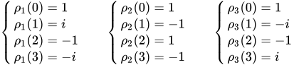






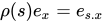

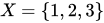
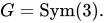
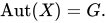

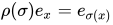



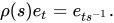





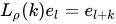

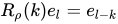
![{\displaystyle K[G]}](https://wikimedia.org/api/rest_v1/media/math/render/svg/083a999799be375d1cbc5c62575915924775f275)

![{\displaystyle f\in K[G]}](https://wikimedia.org/api/rest_v1/media/math/render/svg/30bcdaf430604d2257ca4ab6337e2aa366ce839d)


![{\displaystyle \mathbb {C} [G]}](https://wikimedia.org/api/rest_v1/media/math/render/svg/72c0617967677acd130f2710308f9d00a288efc5)



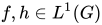
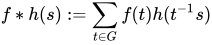


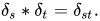
![{\displaystyle \mathbb {C} [G],}](https://wikimedia.org/api/rest_v1/media/math/render/svg/fc160488569e6cb6a4978e1e3ccf18766ed0835d)


![{\displaystyle \mathbb {C} [G].}](https://wikimedia.org/api/rest_v1/media/math/render/svg/ccbd501df0fe67f8c21392b50f9709da854cb472)
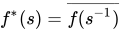



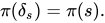





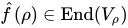

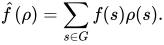

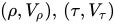
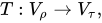

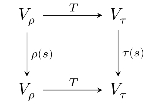










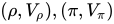
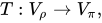







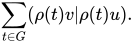













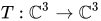








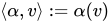




(s_{1},s_{2})(v_{1},v_{2}):=\rho _{1}(s_{1})v_{1}\oplus \rho _{2}(s_{2})v_{2}\end{cases}}}](https://wikimedia.org/api/rest_v1/media/math/render/svg/cac4efc7d528b4d9d0c811273c4589cd1fa17962)




![{\displaystyle {\begin{cases}\rho _{1}:\mathbb {Z} /2\mathbb {Z} \to {\text{GL}}_{2}(\mathbb {C} )\\[4pt]\rho _{1}(1)={\begin{pmatrix}0&-i\\i&0\end{pmatrix}}\end{cases}}\qquad \qquad {\begin{cases}\rho _{2}:\mathbb {Z} /3\mathbb {Z} \to {\text{GL}}_{3}(\mathbb {C} )\\[6pt]\rho _{2}(1)={\begin{pmatrix}1&0&\omega \\0&\omega &0\\0&0&\omega ^{2}\end{pmatrix}}\end{ケース}}}](https://wikimedia.org/api/rest_v1/media/math/render/svg/2e3f54de71e01a5dc4f85b982e627c8916756549)
![{\displaystyle {\begin{cases}\rho _{1}\oplus \rho _{2}:\mathbb {Z} /2\mathbb {Z} \times \mathbb {Z} /3\mathbb {Z} \to {\text{GL}}\left(\mathbb {C} ^{2}\oplus \mathbb {C} ^{3}\right)\\[6pt]\left(\rho _{1}\oplus \rho _{2}\right)(k,l)={\begin{pmatrix}\rho _{1}(k)&0\\0&\rho _{2}(l)\end{pmatrix}}&k\in \mathbb {Z} /2\mathbb {Z} ,l\in \mathbb {Z} /3\mathbb {Z} \end{ケース}}}](https://wikimedia.org/api/rest_v1/media/math/render/svg/14d1e108f72cc9bb9e0f65a57b7bc3baefc92d60)
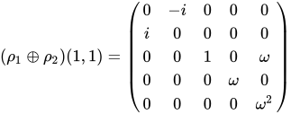








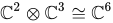
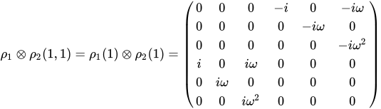









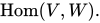
















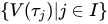
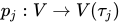
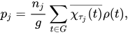
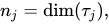


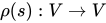








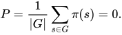



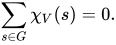















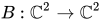
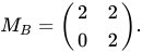

















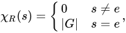










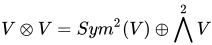




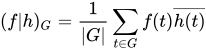

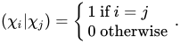

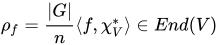








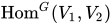







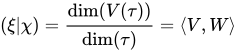


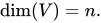



![{\displaystyle \mathbb {C} [G]\cong \oplus _{j}{\text{End}}(W_{j})}](https://wikimedia.org/api/rest_v1/media/math/render/svg/c584d2b52c2ec4e1385588ead185634022e72f5b)







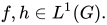





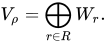




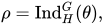


![{\displaystyle \mathbb {C} [H]}](https://wikimedia.org/api/rest_v1/media/math/render/svg/1370654a9e95009d0f9d4333150b3dd9c3fa906a)
![{\displaystyle V=\mathbb {C} [G]\otimes _{\mathbb {C} [H]}W,}](https://wikimedia.org/api/rest_v1/media/math/render/svg/51624468bd57289de42ba50c0d6f9c6dbf3b4dcb)




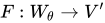


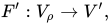



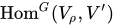



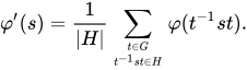

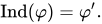








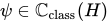
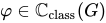

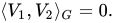



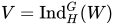

















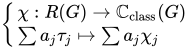


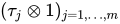






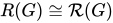























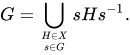


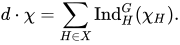













![{\displaystyle {\begin{cases}\rho :G\to {\text{GL}}_{2}(\mathbb {C} )\\[4pt]\rho (\pm 1)={\begin{pmatrix}\pm 1&0\\0&\pm 1\end{pmatrix}},\quad \rho (\pm i)={\begin{pmatrix}\pm i&0\\0&\mp i\end{pmatrix}},\quad \rho (\pm j)={\begin{pmatrix}0&\pm i\\\pm i&0\end{pmatrix}}\end{cases}}}](https://wikimedia.org/api/rest_v1/media/math/render/svg/1951a54fb63c603e82bdbf5996648da4862bec5e)

![{\displaystyle {\begin{cases}\rho :\mathbb {Z} /m\mathbb {Z} \to {\text{GL}}_{2}(\mathbb {R} )\\[4pt]\rho (k)={\begin{pmatrix}\cos \left({\frac {2\pi ik}{m}}\right)&\sin \left({\frac {2\pi ik}{m}}\right)\\-\sin \left({\frac {2\pi ik}{m}}\right)&\cos \left({\frac {2\pi ik}{m}}\right)\end{pmatrix}}\end{cases}}}](https://wikimedia.org/api/rest_v1/media/math/render/svg/faa9aaf2bc6c2828a4f69cabe8b0ae5d3f1209b7)

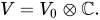


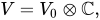












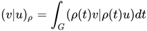









![{\displaystyle L^{2}(G)\cong L^{1}(G)\cong \mathbb {C} [G].}](https://wikimedia.org/api/rest_v1/media/math/render/svg/6f20ae0eb5423391ba55c15f6e10c380d862a00c)






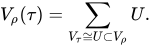







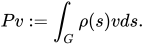

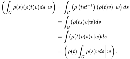





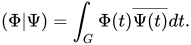
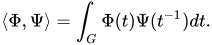















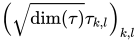



![{\displaystyle {\begin{cases}\Phi \mapsto \sum _{\tau \in {\widehat {G}}}\tau (\Phi )\\[5pt]\tau (\Phi )=\int _{G}\Phi (t)\tau (t)dt\in {\text{End}}(V_{\tau })\end{cases}}}](https://wikimedia.org/api/rest_v1/media/math/render/svg/a07ad8edebba16703e8df32819e703402b95d9f0)