Likelihood function

A likelihood function (often simply called the likelihood) measures how well a statistical model explains observed data by calculating the probability of seeing that data under different parameter values of the model. It is constructed from the joint probability distribution of the random variable that (presumably) generated the observations.^[1]^[2]^[3] When evaluated on the actual data points, it becomes a function solely of the model parameters.

In maximum likelihood estimation, the model parameter(s) or argument that maximizes the likelihood function serves as a point estimate for the unknown parameter, while the Fisher information (often approximated by the likelihood's Hessian matrix at the maximum) gives an indication of the estimate's precision.

In contrast, in Bayesian statistics, the estimate of interest is the converse of the likelihood, the so-called posterior probability of the parameter given the observed data, which is calculated via Bayes' rule.^[4]

Definition

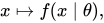
The likelihood function, parameterized by a (possibly multivariate) parameter ${\textstyle \theta }$ , is usually defined differently for discrete and continuous probability distributions (a more general definition is discussed below). Given a probability density or mass function

$x\mapsto f(x\mid \theta ),$

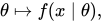
where ${\textstyle x}$ is a realization of the random variable ${\textstyle X}$ , the likelihood function is $\theta \mapsto f(x\mid \theta ),$ often written ${\mathcal {L}}(\theta \mid x).$

In other words, when ${\textstyle f(x\mid \theta )}$ is viewed as a function of ${\textstyle x}$ with ${\textstyle \theta }$ fixed, it is a probability density function, and when viewed as a function of ${\textstyle \theta }$ with ${\textstyle x}$ fixed, it is a likelihood function. In the frequentist paradigm, the notation ${\textstyle f(x\mid \theta )}$ is often avoided and instead ${\textstyle f(x;\theta )}$ or ${\textstyle f(x,\theta )}$ are used to indicate that ${\textstyle \theta }$ is regarded as a fixed unknown quantity rather than as a random variable being conditioned on.

The likelihood function does not specify the probability that ${\textstyle \theta }$ is the truth, given the observed sample ${\textstyle X=x}$ . Such an interpretation is a common error, with potentially disastrous consequences (see prosecutor's fallacy).

Discrete probability distribution

Let ${\textstyle X}$ be a discrete random variable with probability mass function ${\textstyle p}$ depending on a parameter ${\textstyle \theta }$ . Then the function

${\mathcal {L}}(\theta \mid x)=p_{\theta }(x)=P_{\theta }(X=x)={\text{Pr}}\{X=x\mid \Theta =\theta \},$

considered as a function of ${\textstyle \theta }$ , a possible value of the deterministic but unknown parameter ${\textstyle \Theta }$ , is the likelihood function, given the outcome ${\textstyle x}$ of the random variable ${\textstyle X}$ . Sometimes the probability of "the value ${\textstyle x}$ of ${\textstyle X}$ for the parameter value ${\textstyle \theta }$ " is written as $P (X = x | θ)$ or $P (X = x; θ)$ . The likelihood is the probability that a particular outcome ${\textstyle x}$ is observed when the true value of the parameter is ${\textstyle \theta }$ , equivalent to the probability mass on ${\textstyle x}$ ; it is not a probability density over the parameter ${\textstyle \theta }$ . The likelihood, ${\textstyle {\mathcal {L}}(\theta \mid x)}$ , should not be confused with ${\textstyle P(\theta \mid x)}$ , which is the posterior probability of ${\textstyle \theta }$ given the data ${\textstyle x}$ .

Example

Figure 1. The likelihood function ( ${\textstyle p_{\text{H}}^{2}}$ ) for the probability of a coin landing heads-up (without prior knowledge of the coin's fairness), given that we have observed HH.

Figure 1. The likelihood function ( ${\textstyle p_{\text{H}}^{2}}$ ) for the probability of a coin landing heads-up (without prior knowledge of the coin's fairness), given that we have observed HH.

Figure 2. The likelihood function ( ${\textstyle p_{\text{H}}^{2}(1-p_{\text{H}})}$ ) for the probability of a coin landing heads-up (without prior knowledge of the coin's fairness), given that we have observed HHT.

Figure 2. The likelihood function ( ${\textstyle p_{\text{H}}^{2}(1-p_{\text{H}})}$ ) for the probability of a coin landing heads-up (without prior knowledge of the coin's fairness), given that we have observed HHT.

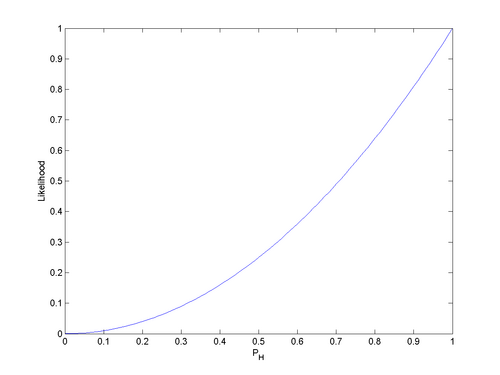
Consider a simple statistical model of a coin flip: a single parameter ${\textstyle p_{\text{H}}}$ that expresses the "fairness" of the coin. The parameter is the probability that a coin lands heads up ("H") when tossed. ${\textstyle p_{\text{H}}}$ can take on any value within the range 0.0 to 1.0. For a perfectly fair coin, ${\textstyle p_{\text{H}}=0.5}$ .

Imagine flipping a fair coin twice, and observing two heads in two tosses ("HH"). Assuming that each successive coin flip is i.i.d., then the probability of observing HH is

$P({\text{HH}}\mid p_{\text{H}}=0.5)=0.5^{2}=0.25.$

Equivalently, the likelihood of observing "HH" assuming ${\textstyle p_{\text{H}}=0.5}$ is

${\mathcal {L}}(p_{\text{H}}=0.5\mid {\text{HH}})=0.25.$

This is not the same as saying that ${\textstyle P(p_{\text{H}}=0.5\mid {\text{HH}})=0.25}$ , a conclusion which could only be reached via Bayes' theorem given knowledge about the marginal probabilities ${\textstyle P(p_{\text{H}}=0.5)}$ and ${\textstyle P({\text{HH}})}$ .

Now suppose that the coin is not a fair coin, but instead that ${\textstyle p_{\text{H}}=0.3}$ . Then the probability of two heads on two flips is

$P({\text{HH}}\mid p_{\text{H}}=0.3)=0.3^{2}=0.09.$

Hence

${\mathcal {L}}(p_{\text{H}}=0.3\mid {\text{HH}})=0.09.$

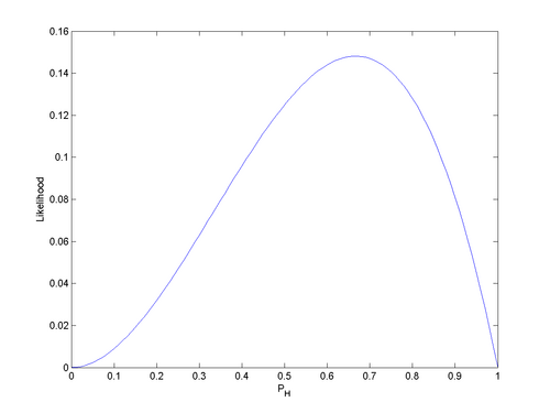
More generally, for each value of ${\textstyle p_{\text{H}}}$ , we can calculate the corresponding likelihood. The result of such calculations is displayed in Figure 1. The integral of ${\textstyle {\mathcal {L}}}$ over [0, 1] is 1/3; likelihoods need not integrate or sum to one over the parameter space.

Continuous probability distribution

Let ${\textstyle X}$ be a random variable following an absolutely continuous probability distribution with density function ${\textstyle f}$ (a function of ${\textstyle x}$ ) which depends on a parameter ${\textstyle \theta }$ . Then the function

${\mathcal {L}}(\theta \mid x)=f_{\theta }(x),$

considered as a function of ${\textstyle \theta }$ , is the likelihood function (of ${\textstyle \theta }$ , given the outcome ${\textstyle X=x}$ ). Again, ${\textstyle {\mathcal {L}}}$ is not a probability density or mass function over ${\textstyle \theta }$ , despite being a function of ${\textstyle \theta }$ given the observation ${\textstyle X=x}$ .

Relationship between the likelihood and probability density functions

The use of the probability density in specifying the likelihood function above is justified as follows. Given an observation ${\textstyle x_{j}}$ , the likelihood for the interval ${\textstyle [x_{j},x_{j}+h]}$ , where ${\textstyle h>0}$ is a constant, is given by ${\textstyle {\mathcal {L}}(\theta \mid x\in [x_{j},x_{j}{+}h])}$ . Observe that $\mathop {\operatorname {arg\,max} } _{\theta }{\mathcal {L}}(\theta \mid x\in [x_{j},x_{j}{+}h])=\mathop {\operatorname {arg\,max} } _{\theta }{\frac {1}{h}}{\mathcal {L}}(\theta \mid x\in [x_{j},x_{j}{+}h]),$ since ${\textstyle h}$ is positive and constant. Because ${\begin{aligned}\mathop {\operatorname {arg\,max} } _{\theta }{\frac {1}{h}}{\mathcal {L}}(\theta \mid x\in [x_{j},x_{j}{+}h])&=\mathop {\operatorname {arg\,max} } _{\theta }{\frac {1}{h}}\Pr(x_{j}\leq x\leq x_{j}{+}h\mid \theta )\\&=\mathop {\operatorname {arg\,max} } _{\theta }{\frac {1}{h}}\int _{x_{j}}^{x_{j}+h}f(x\mid \theta )\,dx,\end{aligned}}$

where ${\textstyle f(x\mid \theta )}$ is the probability density function, it follows that

$\mathop {\operatorname {arg\,max} } _{\theta }{\mathcal {L}}(\theta \mid x\in [x_{j},x_{j}+h])=\mathop {\operatorname {arg\,max} } _{\theta }{\frac {1}{h}}\int _{x_{j}}^{x_{j}+h}f(x\mid \theta )\,dx.$

The first fundamental theorem of calculus provides that $\lim _{h\to 0^{+}}{\frac {1}{h}}\int _{x_{j}}^{x_{j}+h}f(x\mid \theta )\,dx=f(x_{j}\mid \theta ).$

Then ${\begin{aligned}\mathop {\operatorname {arg\,max} } _{\theta }{\mathcal {L}}(\theta \mid x_{j})&=\mathop {\operatorname {arg\,max} } _{\theta }\left[\lim _{h\to 0^{+}}{\mathcal {L}}(\theta \mid x\in [x_{j},\,x_{j}{+}h])\right]\\[4pt]&=\mathop {\operatorname {arg\,max} } _{\theta }\left[\lim _{h\to 0^{+}}{\frac {1}{h}}\int _{x_{j}}^{x_{j}+h}f(x\mid \theta )\,dx\right]\\[4pt]&=\mathop {\operatorname {arg\,max} } _{\theta }f(x_{j}\mid \theta ).\end{aligned}}$

Therefore, $\mathop {\operatorname {arg\,max} } _{\theta }{\mathcal {L}}(\theta \mid x_{j})=\mathop {\operatorname {arg\,max} } _{\theta }f(x_{j}\mid \theta ),$ and so maximizing the probability density at ${\textstyle x_{j}}$ amounts to maximizing the likelihood of the specific observation ${\textstyle x_{j}}$ .

In general

In measure-theoretic probability theory, the density function is defined as the Radon–Nikodym derivative of the probability distribution relative to a common dominating measure.^[5] The likelihood function is this density interpreted as a function of the parameter, rather than the random variable.^[6] Thus, we can construct a likelihood function for any distribution, whether discrete, continuous, a mixture, or otherwise. (Likelihoods are comparable, e.g. for parameter estimation, only if they are Radon–Nikodym derivatives with respect to the same dominating measure.)

The above discussion of the likelihood for discrete random variables uses the counting measure, under which the probability density at any outcome equals the probability of that outcome.

Likelihoods for mixed continuous–discrete distributions

The above can be extended in a simple way to allow consideration of distributions which contain both discrete and continuous components. Suppose that the distribution consists of a number of discrete probability masses ${\textstyle p_{k}(\theta )}$ and a density ${\textstyle f(x\mid \theta )}$ , where the sum of all the ${\textstyle p}$ 's added to the integral of ${\textstyle f}$ is always one. Assuming that it is possible to distinguish an observation corresponding to one of the discrete probability masses from one which corresponds to the density component, the likelihood function for an observation from the continuous component can be dealt with in the manner shown above. For an observation from the discrete component, the likelihood function for an observation from the discrete component is simply ${\mathcal {L}}(\theta \mid x)=p_{k}(\theta ),$ where ${\textstyle k}$ is the index of the discrete probability mass corresponding to observation ${\textstyle x}$ , because maximizing the probability mass (or probability) at ${\textstyle x}$ amounts to maximizing the likelihood of the specific observation.

The fact that the likelihood function can be defined in a way that includes contributions that are not commensurate (the density and the probability mass) arises from the way in which the likelihood function is defined up to a constant of proportionality, where this "constant" can change with the observation ${\textstyle x}$ , but not with the parameter ${\textstyle \theta }$ .

Regularity conditions

In the context of parameter estimation, the likelihood function is usually assumed to obey certain conditions, known as regularity conditions. These conditions are assumed in various proofs involving likelihood functions, and need to be verified in each particular application. For maximum likelihood estimation, the existence of a global maximum of the likelihood function is of the utmost importance. By the extreme value theorem, it suffices that the likelihood function is continuous on a compact parameter space for the maximum likelihood estimator to exist.^[7] While the continuity assumption is usually met, the compactness assumption about the parameter space is often not, as the bounds of the true parameter values might be unknown. In that case, concavity of the likelihood function plays a key role.

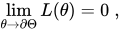
More specifically, if the likelihood function is twice continuously differentiable on the k-dimensional parameter space ${\textstyle \Theta }$ assumed to be an open connected subset of ${\textstyle \mathbb {R} ^{k}\,,}$ there exists a unique maximum ${\textstyle {\hat {\theta }}\in \Theta }$ if the matrix of second partials $\mathbf {H} (\theta )\equiv \left[\,{\frac {\partial ^{2}L}{\partial \theta _{i}\,\partial \theta _{j}}}\,\right]_{i,j=1,1}^{n_{\mathrm {i} },n_{\mathrm {j} }}\;$ is negative definite for every ${\textstyle \theta \in \Theta }$ at which the gradient ${\textstyle \nabla L\equiv \left[{\frac {\partial L}{\partial \theta _{i}}}\right]_{i=1}^{n_{\mathrm {i} }}}$ vanishes, and if the likelihood function approaches a constant on the boundary of the parameter space, ${\textstyle \partial \Theta ,}$ i.e., $\lim _{\theta \to \partial \Theta }L(\theta )=0\;,$ which may include the points at infinity if ${\textstyle \Theta }$ is unbounded. Mäkeläinen and co-authors prove this result using Morse theory while informally appealing to a mountain pass property.^[8] Mascarenhas restates their proof using the mountain pass theorem.^[9]

In the proofs of consistency and asymptotic normality of the maximum likelihood estimator, additional assumptions are made about the probability densities that form the basis of a particular likelihood function. These conditions were first established by Chanda.^[10] In particular, for almost all ${\textstyle x}$ , and for all ${\textstyle \,\theta \in \Theta \,,}$ ${\frac {\partial \log f}{\partial \theta _{r}}}\,,\quad {\frac {\partial ^{2}\log f}{\partial \theta _{r}\partial \theta _{s}}}\,,\quad {\frac {\partial ^{3}\log f}{\partial \theta _{r}\,\partial \theta _{s}\,\partial \theta _{t}}}\,$ exist for all ${\textstyle \,r,s,t=1,2,\ldots ,k\,}$ in order to ensure the existence of a Taylor expansion. Second, for almost all ${\textstyle x}$ and for every ${\textstyle \,\theta \in \Theta \,}$ it must be that $\left|{\frac {\partial f}{\partial \theta _{r}}}\right|<F_{r}(x)\,,\quad \left|{\frac {\partial ^{2}f}{\partial \theta _{r}\,\partial \theta _{s}}}\right|<F_{rs}(x)\,,\quad \left|{\frac {\partial ^{3}f}{\partial \theta _{r}\,\partial \theta _{s}\,\partial \theta _{t}}}\right|<H_{rst}(x)$ where ${\textstyle H}$ is such that ${\textstyle \,\int _{-\infty }^{\infty }H_{rst}(z)\,dz\leq M<\infty \;.}$ This boundedness of the derivatives is needed to allow for differentiation under the integral sign. And lastly, it is assumed that the information matrix, $\mathbf {I} (\theta )=\int _{-\infty }^{\infty }{\frac {\partial \log f}{\partial \theta _{r}}}\ {\frac {\partial \log f}{\partial \theta _{s}}}\ f\,dz$ is positive definite and ${\textstyle \,\left|\mathbf {I} (\theta )\right|\,}$ is finite. This ensures that the score has a finite variance.^[11]

上記の条件は十分条件ではあるが、必要条件ではない。つまり、これらの正則性条件を満たさないモデルは、上述の特性の最尤推定量を持つ場合もあれば、持たない場合もある。さらに、観測値が独立または同一分布に従わない場合には、追加の特性を仮定する必要があるかもしれない。

ベイズ統計学では、事後確率の漸近正規性を証明するため、尤度関数にほぼ同一の正則性条件が課せられ、^{[ 12 ]}^{[ 13 ]}したがって、大標本における事後確率のラプラス近似を正当化する。^{[ 14 ]}

尤度比と相対尤度

尤度比

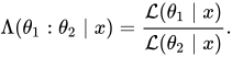
尤度比とは、指定された2つの尤度の比であり、多くの場合次のように表記されます。 $\Lambda (\theta _{1}:\theta _{2}\mid x)={\frac {{\mathcal {L}}(\theta _{1}\mid x)}{{\mathcal {L}}(\theta _{2}\mid x)}}.$

尤度比は尤度統計学の中心となる概念である。尤度の法則によれば、データ（証拠とみなされる）が一方のパラメータ値を他方のパラメータ値よりもどの程度支持しているかは、尤度比によって測定される。

頻度論的推論では、尤度比は検定統計量の基礎であり、いわゆる尤度比検定である。ネイマン・ピアソン補題によれば、これは与えられた有意水準で2つの単純な仮説を比較するための最も強力な検定である。他の多くの検定は、尤度比検定またはその近似と見なすことができる。^[¹⁵^]検定統計量として考えられる対数尤度比の漸近分布は、ウィルクスの定理によって与えられる。

尤度比はベイズ推論においても中心的な重要性を持ち、ベイズ因子として知られ、ベイズの定理で使用されます。オッズの観点から述べると、ベイズの定理は、2 つの選択肢の事後オッズが、 $A_{1}$ そして $A_{2}$ ⁠、イベントが与えられた場合⁠ $B$ ⁠ は、事前オッズに尤度比を掛けたものです。数式で表すと次のようになります。 $O(A_{1}:A_{2}\mid B)=O(A_{1}:A_{2})\cdot \Lambda (A_{1}:A_{2}\mid B).$

尤度比はAICに基づく統計手法では直接使用されません。代わりに、モデルの相対尤度が使用されます（下記参照）。

根拠に基づいた医療では、診断検査を実施する価値を評価するために、診断検査において尤度比が用いられる。

相対尤度関数

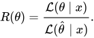
尤度関数の実際の値はサンプルに依存するため、標準化された尺度を用いると便利な場合が多い。パラメータ $θの$ 最尤推定値が次のようになると仮定する。 ${\textstyle {\hat {\theta }}}$ 他の $θ$ 値の相対的な妥当性は、それらの他の値の尤度と、 ${\textstyle {\hat {\theta }}}$ $θ$ の相対尤度は次のように定義されます^[¹⁶^]^[¹⁷^]^[¹⁸^]^[¹⁹^]^[²⁰^] $R(\theta )={\frac {{\mathcal {L}}(\theta \mid x)}{{\mathcal {L}}({\hat {\theta }}\mid x)}}.$ したがって、相対尤度は、固定分母を持つ尤度比（上記で説明した）である。 ${\textstyle {\mathcal {L}}({\hat {\theta }})}$ これは、最大確率が1になるように標準化することに相当します。

可能性領域

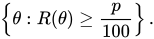
尤度領域とは、相対尤度が与えられた閾値以上である $θ$ のすべての値の集合です。パーセンテージで表すと、 $θ$ の $p$ %尤度領域は次のように定義されます^[¹⁶^]^[¹⁸^]^[²¹^{] 。}

$\left\{\theta :R(\theta )\geq {\frac {p}{100}}\right\}.$

$θ$ が単一の実数パラメータである場合、 $p$ %尤度領域は通常、実数値の区間で構成されます。領域が区間で構成されている場合、それは尤度区間と呼ばれます。^{[ 16 ]}^{[ 18 ]}^{[ 22 ]}

尤度区間、より一般的には尤度領域は、尤度統計学における区間推定に用いられます。これらは、頻度統計学における信頼区間やベイズ統計学における信用区間に類似しています。尤度区間は、包含確率（頻度主義）や事後確率（ベイズ主義）ではなく、相対尤度の観点から直接解釈されます。

モデルが与えられた場合、尤度区間は信頼区間と比較できます。θ が単一の実数パラメータである場合 $、$ 特定の条件下では、 $θ$ の 14.65% 尤度区間 (約 1:7 の尤度)は 95% 信頼区間 (19/20 のカバレッジ確率) と同じになります。^{[ 16 ]}^{[ 21 ]}対数尤度の使用に適した少し異なる定式化 (ウィルクスの定理を参照) では、検定統計量は対数尤度の差の 2 倍であり、検定統計量の確率分布は、2 つのモデル間の自由度の差に等しい自由度 (df) を持つカイ二乗分布に近似します (したがって、 $e$ ^{− 2}尤度区間は 0.954 信頼区間と同じです。df の差が 1 であると仮定します)。^{[ 21 ]}^{[ 22 ]}

不要なパラメータを排除する尤度

多くの場合、尤度は複数のパラメータの関数ですが、関心は 1 つまたはせいぜい数個のパラメータの推定に集中し、他のパラメータは不要パラメータとみなされます。このような不要パラメータを排除して尤度を関心のあるパラメータ (または複数のパラメータ) の関数として記述できるようにするために、いくつかの代替アプローチが開発されています。主なアプローチは、プロファイル尤度、条件付き尤度、周辺尤度です。^{[ 23 ]}^{[ 24 ]}これらのアプローチは、グラフを可能にするために、高次元の尤度曲面を 1 つまたは 2 つの関心のあるパラメータに縮小する必要がある場合にも役立ちます。

プロファイルの可能性

パラメータのサブセットに対する尤度関数を集中させることで次元を削減することが可能であり、そのためには、不要なパラメータを関心のあるパラメータの関数として表現し、それらを尤度関数に置き換える必要がある。^{[ 25 ]}^{[ 26 ]}一般に、パラメータベクトルに依存する尤度関数については、 ${\textstyle \mathbf {\theta } }$ 分割できる ${\textstyle \mathbf {\theta } =\left(\mathbf {\theta } _{1}:\mathbf {\theta } _{2}\right)}$ 、そして対応関係がある場合 ${\textstyle \mathbf {\hat {\theta }} _{2}=\mathbf {\hat {\theta }} _{2}\left(\mathbf {\theta } _{1}\right)}$ 明示的に決定することができ、集中により元の最大化問題の計算負荷が軽減される。 ^{[ 27 ]}

例えば、誤差が正規分布する線形回帰では、 ${\textstyle \mathbf {y} =\mathbf {X} \beta +u}$ 係数ベクトルは以下のように分割できます。 ${\textstyle \beta =\left[\beta _{1}:\beta _{2}\right]}$ （そして結果として設計マトリックスも） ${\textstyle \mathbf {X} =\left[\mathbf {X} _{1}:\mathbf {X} _{2}\right]}$ ）に関して最大化する ${\textstyle \beta _{2}}$ 最適な値関数が得られる ${\textstyle \beta _{2}(\beta _{1})=\left(\mathbf {X} _{2}^{\mathsf {T}}\mathbf {X} _{2}\right)^{-1}\mathbf {X} _{2}^{\mathsf {T}}\left(\mathbf {y} -\mathbf {X} _{1}\beta _{1}\right)}$ この結果を用いると、 ${\textstyle \beta _{1}}$ すると、次のように導き出せる。 ${\hat {\beta }}_{1}=\left(\mathbf {X} _{1}^{\mathsf {T}}\left(\mathbf {I} -\mathbf {P} _{2}\right)\mathbf {X} _{1}\right)^{-1}\mathbf {X} _{1}^{\mathsf {T}}\left(\mathbf {I} -\mathbf {P} _{2}\right)\mathbf {y}$ どこ ${\textstyle \mathbf {P} _{2}=\mathbf {X} _{2}\left(\mathbf {X} _{2}^{\mathsf {T}}\mathbf {X} _{2}\right)^{-1}\mathbf {X} _{2}^{\mathsf {T}}}$ is the projection matrix of ${\textstyle \mathbf {X} _{2}}$ . This result is known as the Frisch–Waugh–Lovell theorem.

Since graphically the procedure of concentration is equivalent to slicing the likelihood surface along the ridge of values of the nuisance parameter ${\textstyle \beta _{2}}$ that maximizes the likelihood function, creating an isometric profile of the likelihood function for a given ${\textstyle \beta _{1}}$ , the result of this procedure is also known as profile likelihood.^[28]^[29] In addition to being graphed, the profile likelihood can also be used to compute confidence intervals that often have better small-sample properties than those based on asymptotic standard errors calculated from the full likelihood.^[30]^[31]

Conditional likelihood

Sometimes it is possible to find a sufficient statistic for the nuisance parameters, and conditioning on this statistic results in a likelihood which does not depend on the nuisance parameters.^[32]

One example occurs in 2×2 tables, where conditioning on all four marginal totals leads to a conditional likelihood based on the non-central hypergeometric distribution. This form of conditioning is also the basis for Fisher's exact test.

Marginal likelihood

Sometimes we can remove the nuisance parameters by considering a likelihood based on only part of the information in the data, for example by using the set of ranks rather than the numerical values. Another example occurs in linear mixed models, where considering a likelihood for the residuals only after fitting the fixed effects leads to residual maximum likelihood estimation of the variance components.

Partial likelihood

A partial likelihood is an adaption of the full likelihood such that only a part of the parameters (the parameters of interest) occur in it.^[33] It is a key component of the proportional hazards model: using a restriction on the hazard function, the likelihood does not contain the shape of the hazard over time.

Products of likelihoods

The likelihood, given two or more independent events, is the product of the likelihoods of each of the individual events: $\Lambda (A\mid X_{1}\land X_{2})=\Lambda (A\mid X_{1})\cdot \Lambda (A\mid X_{2}).$ This follows from the definition of independence in probability: the probabilities of two independent events happening, given a model, is the product of the probabilities.

これは、事象が独立同分布の確率変数から生じる場合、例えば独立観測や復元抽出によるサンプリングの場合に特に重要です。このような状況では、尤度関数は個々の尤度関数の積に分解されます。

空の積の値は1であり、これは事象が発生しない場合の尤度が1であることに対応します。つまり、データが与えられる前は、尤度は常に1です。これはベイズ統計における一様事前分布に似ていますが、尤度統計では尤度は積分されないため、これは不適切な事前分布ではありません。

対数尤度

対数尤度関数は尤度関数の対数であり、小文字の $l$ または⁠で表されることが多い。 $\ell$ 大文字の $L$ と対比して、 ${\textstyle {\mathcal {L}}}$ 尤度については、対数は厳密に増加する関数であるため、尤度を最大化することは対数尤度を最大化することと同等です。しかし、実際的な目的においては、最尤推定では対数尤度関数を使用する方が便利です。特に、最も一般的な確率分布（特に指数族）は対数的に凹であるだけであり、^{[ 34 ]}^{[ 35 ]}目的関数の凹性が最大化において重要な役割を果たします。

各事象が独立していることを前提とすると、交差の全体的な対数尤度は、個々の事象の対数尤度の合計に等しくなります。これは、全体的な対数確率が個々の事象の対数確率の合計であるという事実と類似しています。この数学的な利便性に加えて、対数尤度の加算プロセスには、データからの「支持」としてよく表現されるように、直感的な解釈があります。最尤推定のために対数尤度を使用してパラメータを推定する場合、各データポイントは全体の対数尤度に加算されます。データは推定されたパラメータを支持する証拠と見なすことができるため、このプロセスは「独立した証拠からの支持が加算される」と解釈でき、対数尤度は「証拠の重み」となります。負の対数確率を情報量または驚き度として解釈すると、ある事象が与えられた場合のモデルの支持度（対数尤度）は、そのモデルが与えられた場合の事象の驚き度の負の値になります。つまり、その事象がモデルが与えられた場合に驚き度が低いほど、モデルはその事象によって支持されると言えます。

尤度比の対数は、対数尤度の差に等しい。 $\log {\frac {{\mathcal {L}}(A)}{{\mathcal {L}}(B)}}=\log {\mathcal {L}}(A)-\log {\mathcal {L}}(B)=\ell (A)-\ell (B).$

事象が発生しない場合の尤度が1であるのと同様に、事象が発生しない場合の対数尤度は0であり、これは空の合計値に対応します。つまり、データがなければ、どのモデルも支持されません。

グラフ

対数尤度のグラフは、（単変量の場合）サポート曲線と呼ばれます。[ 36 ]多変量^の^場合^、この概念はパラメータ空間上のサポート曲面に一般化されます。これは分布のサポートと関連がありますが、それとは異なります。

この用語は、統計的仮説検定の文脈でAWF エドワーズ^{[ 36 ]}によって造語されました。つまり、データがテストされている仮説 (またはパラメータ値) のうちの 1 つを他の仮説よりも「支持」しているかどうかということです。

グラフにプロットされている対数尤度関数は、スコア（対数尤度の勾配）とフィッシャー情報量（対数尤度の曲率）の計算に使用されます。したがって、このグラフは最尤推定法と尤度比検定の文脈において直接的な解釈が可能です。

尤度方程式

対数尤度関数が滑らかである場合、パラメータに関するその勾配はスコアとして知られ、次のように表されます。 ${\textstyle s_{n}(\theta )\equiv \nabla _{\theta }\ell _{n}(\theta )}$ が存在し、微分計算の適用を可能にします。微分可能な関数を最大化する基本的な方法は、停留点（導関数がゼロになる点）を見つけることです。和の導関数は導関数の和に等しいですが、積の導関数には積の法則が必要なので、独立事象の尤度よりも独立事象の対数尤度の停留点を計算する方が簡単です。

スコア関数の停留点によって定義される方程式は、最尤推定量の推定方程式として機能する。 $s_{n}(\theta )=\mathbf {0}$ その意味で、最尤推定量は暗黙のうちに次の値によって定義される。 ${\textstyle \mathbf {0} }$ 逆関数の ${\textstyle s_{n}^{-1}:\mathbb {E} ^{d}\to \Theta }$ 、どこ ${\textstyle \mathbb {E} ^{d}}$ はd次元ユークリッド空間であり、 ${\textstyle \Theta }$ はパラメータ空間である。逆関数定理を用いると、次のことが示される。 ${\textstyle s_{n}^{-1}}$ オープンな近隣地域で明確に定義されています ${\textstyle \mathbf {0} }$ 確率は1に近づき、 ${\textstyle {\hat {\theta }}_{n}=s_{n}^{-1}(\mathbf {0} )}$ は、 ${\textstyle \theta }$ 結果として、数列が存在する ${\textstyle \left\{{\hat {\theta }}_{n}\right\}}$ そのため ${\textstyle s_{n}({\hat {\theta }}_{n})=\mathbf {0} }$ 漸近的にほぼ確実に、そして ${\textstyle {\hat {\theta }}_{n}\xrightarrow {\text{p}} \theta _{0}}$ ^{[ 37 ]}ロルの定理を用いて同様の結果を確立することができる。^{[ 38 ]}^{[ 39 ]}

2階微分を評価したところ、 ${\textstyle {\hat {\theta }}}$ フィッシャー情報として知られるこの値は、尤度曲面の曲率を決定し、^{[ 40 ]}推定値の精度を示します。 ^{[ 41 ]}

指数型ファミリー

対数尤度は、多くの一般的なパラメトリック確率分布を含む指数分布族にも特に有用です。指数分布族の確率分布関数（したがって尤度関数）は、指数を含む因子の積を含んでいます。このような関数の対数は積の和であり、元の関数よりも微分が容易です。

指数族とは、確率密度関数が次の形式である分布族のことである（一部の関数では、次のように書くことができる）。 ${\textstyle \langle -,-\rangle }$ 内積の場合）：

$p(x\mid {\boldsymbol {\theta }})=h(x)\exp {\Big (}\langle {\boldsymbol {\eta }}({\boldsymbol {\theta }}),\mathbf {T} (x)\rangle -A({\boldsymbol {\theta }}){\Big )}.$

これらの各項には解釈がありますが、^{[ a ]}確率から尤度に切り替えて対数を取るだけで、次の合計が得られます。

$\ell ({\boldsymbol {\theta }}\mid x)=\langle {\boldsymbol {\eta }}({\boldsymbol {\theta }}),\mathbf {T} (x)\rangle -A({\boldsymbol {\theta }})+\log h(x).$

の ${\textstyle {\boldsymbol {\eta }}({\boldsymbol {\theta }})}$ そして ${\textstyle h(x)}$ それぞれが座標変換に対応しているため、これらの座標では、指数型分布族の対数尤度は次の単純な式で与えられます。

$\ell ({\boldsymbol {\eta }}\mid x)=\langle {\boldsymbol {\eta }},\mathbf {T} (x)\rangle -A({\boldsymbol {\eta }}).$

言い換えれば、指数型分布族の対数尤度は自然パラメータの内積である。 ${\boldsymbol {\eta }}$ ⁠そして十分統計量 $\mathbf {T} (x)$ 正規化係数（対数分割関数）を差し引いた値 $A({\boldsymbol {\eta }})$ したがって、例えば、十分統計量 $T$ と対数分割関数 $A$ の導関数を取ることによって、最尤推定値を計算できます。

例：ガンマ分布

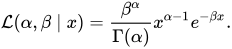
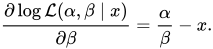
ガンマ分布は2つのパラメータを持つ指数族である。 ${\textstyle \alpha }$ そして ${\textstyle \beta }$ 尤度関数は

${\mathcal {L}}(\alpha ,\beta \mid x)={\frac {\beta ^{\alpha }}{\Gamma (\alpha )}}x^{\alpha -1}e^{-\beta x}.$

最尤推定値を見つける ${\textstyle \beta }$ 単一の観測値に対して ${\textstyle x}$ かなり難しそうに見える。対数の方がずっと扱いやすい。

$\log {\mathcal {L}}(\alpha ,\beta \mid x)=\alpha \log \beta -\log \Gamma (\alpha )+(\alpha -1)\log x-\beta x.\,$

対数尤度を最大化するために、まずに関して偏微分をとります。 ${\textstyle \beta }$ :

${\frac {\partial \log {\mathcal {L}}(\alpha ,\beta \mid x)}{\partial \beta }}={\frac {\alpha }{\beta }}-x.$

複数の独立した観測がある場合 ${\textstyle x_{1},\ldots ,x_{n}}$ すると、結合対数尤度は個々の対数尤度の合計となり、この合計の導関数は各個々の対数尤度の導関数の合計となる。

${\begin{aligned}&{\frac {\partial \log {\mathcal {L}}(\alpha ,\beta \mid x_{1},\ldots ,x_{n})}{\partial \beta }}\\&={\frac {\partial \log {\mathcal {L}}(\alpha ,\beta \mid x_{1})}{\partial \beta }}+\cdots +{\frac {\partial \log {\mathcal {L}}(\alpha ,\beta \mid x_{n})}{\partial \beta }}\\&={\frac {n\alpha }{\beta }}-\sum _{i=1}^{n}x_{i}.\end{aligned}}$

結合対数尤度の最大化手順を完了するために、方程式をゼロに設定して解きます。 ${\textstyle \beta }$ :

${\widehat {\beta }}={\frac {\alpha }{\bar {x}}}.$

ここ ${\textstyle {\widehat {\beta }}}$ は最尤推定値を表し、 ${\textstyle \textstyle {\bar {x}}={\frac {1}{n}}\sum _{i=1}^{n}x_{i}}$ これは観測値の標本平均です。

背景と解釈

歴史的考察

「尤度」という用語は、少なくとも中期英語後期から英語で使われてきました。^{[ 42 ]}数学統計学における特定の関数を指す正式な用語として、ロナルド・フィッシャー[ ⁴³^]が1921年^[⁴⁴^]と1922年^[⁴⁵^]に発表した2つの研究論文で提唱しました。1921年の論文では、今日「尤度区間」と呼ばれるものが導入され、1922年の論文では「最尤法」という用語が導入されました。フィッシャーの言葉を引用すると^、次のようになります。

1922年に私は「尤度」という用語を提案しました。これは、[パラメータ]に関して、尤度は確率ではなく、確率の法則に従わない一方で、[パラメータ]の可能な値の中から合理的に選択するという問題に対して、確率が偶然のゲームにおける事象の予測という問題に対して持つ関係に似た関係を持つという事実に基づいています。…しかし、心理的判断に関して、尤度は確率とある程度似ていますが、この2つの概念は全く異なります。…」^{[ 46 ]}

ロナルド・フィッシャー卿が述べたように、可能性の概念は確率と混同してはならない。

私がこの点を強調するのは、確率と尤度の違いを常に強調してきたにもかかわらず、尤度を一種の確率であるかのように扱う傾向が依然としてあるためです。したがって、最初の結果は、異なるケースに適した2つの異なる合理的信念の尺度が存在するということです。母集団を知っている場合、標本に関する不完全な知識または期待を確率で表現できます。標本を知っている場合、母集団に関する不完全な知識を尤度で表現できます。^{[ 47 ]}

フィッシャーによる統計的尤度の発明は、逆確率と呼ばれる以前の推論形式に対する反動であった。^{[ 48 ]}彼が「尤度」という用語を使用したことで、数学統計学におけるその用語の意味が固定された。

AWF エドワーズ(1972) は、対数尤度比をある仮説に対する別の仮説の相対的な支持の尺度として使用するための公理的基礎を確立しました。支持関数は、尤度関数の自然対数です。これらの用語はどちらも系統発生学で使用されていますが、統計的証拠のトピックの一般的な扱いには採用されていません。^{[ 49 ]}

異なる根拠に基づく解釈

統計学者の間では、統計の基礎が何であるべきかについて合意はありません。基礎として提案されている主なパラダイムは、頻度主義、ベイズ主義、尤度主義、AICベースという4つです。^{[ 50 ]}提案されているそれぞれの基礎において、尤度の解釈は異なります。4つの解釈については、以下のサブセクションで説明します。

頻度主義的解釈

ベイズ解釈

ベイズ推論では、ある命題または確率変数が別の確率変数を与えられた場合の尤度について話すことができます。たとえば、特定のデータまたはその他の証拠が与えられた場合のパラメータ値または統計モデルの尤度(周辺尤度を参照) などです。^{[ 51 ]}^{[ 52 ]}^{[ 53 ]}^{[ 54 ]}尤度関数は同じ実体のままですが、(i)パラメータが与えられた場合のデータの条件付き密度(パラメータは確率変数であるため) および (ii) パラメータ値またはモデルに関するデータによってもたらされる情報の尺度または量という追加の解釈があります。 ^{[ 51 ]}^{[ 52 ]}^{[ 53 ]}^{[ 54 ]}^{[ 55 ]}パラメータ空間またはモデルの集合に確率構造が導入されたことにより、パラメータ値または統計モデルが、与えられたデータに対して大きな尤度値を持つにもかかわらず、低い確率を持つ、またはその逆の可能性があります。^{[ 53 ]}^{[ 55 ]}これは医療の文脈でよく見られます。^{[ 56 ]}ベイズの定理に従うと、条件付き密度として見た場合の尤度は、パラメータの事前確率密度を乗じて正規化することで、事後確率密度が得られます。^{[ 51 ]}^{[ 52 ]}^{[ 53 ]}^{[ 54 ]}^{[ 55 ]}より一般的には、未知の量の尤度は ${\textstyle X}$ 別の未知の量が与えられた場合 ${\textstyle Y}$ 確率に比例する ${\textstyle Y}$ 与えられた ${\textstyle X}$ [ ⁵¹^]^[⁵²^]^[⁵³^]^[⁵⁴^]^[⁵⁵^]

尤度論的解釈

頻度統計学では、尤度関数自体が母集団から抽出した単一の標本を要約する統計量であり、その計算値は、いくつかのパラメータθ ₁ ... θ _pの選択に依存します。ここで、pは既に選択された統計モデルにおけるパラメータの数です。尤度の値は、パラメータの選択に対する評価指標として機能し、利用可能なデータに基づいて、尤度が最大となるパラメータセットが最良の選択となります。

尤度の具体的な計算は、選択されたモデルといくつかのパラメータθの値が、観測されたサンプルが抽出された母集団の頻度分布を正確に近似していると仮定した場合に、観測されたサンプルが割り当てられる確率です。経験的に、実際に観測されたサンプルが起こった事後確率を最大にするようなパラメータを選択するのが良い選択であるというのは理にかなっています。ウィルクスの定理は、推定値のパラメータ値によって生成される尤度の対数と、母集団の「真の」（ただし未知の）パラメータ値によって生成される尤度の対数の差が漸近的に χ ²分布に従うことを示すことで、この経験則を定量化しています。

各独立標本の最尤推定値は、標本抽出された母集団を記述する「真の」パラメータセットの個別の推定値です。多数の独立標本から得られる連続的な推定値は、母集団の「真の」パラメータ値セットがそれらのどこかに隠れている状態で、互いにクラスターを形成します。最尤推定値と隣接するパラメータセットの尤度の対数の差は、座標がパラメータθ ₁ ... θ _pであるプロット上に信頼領域を描くために使用できます。この領域は最尤推定値を囲み、その領域内のすべての点（パラメータセット）は、対数尤度においてある固定値のみ異なります。ウィルクスの定理によって与えられるχ ² 分布は、この領域の対数尤度の差を、母集団の「真の」パラメータセットがその領域内に存在する「信頼度」に変換します。固定対数尤度の差を選択する際のコツは、信頼度を許容できるほど高くしつつ、領域を許容できるほど小さく（推定値の範囲を狭く）することです。

観測データが増えるにつれて、それらを個別の推定値を算出するために用いるのではなく、以前のサンプルと組み合わせて単一の結合サンプルを作成し、その大きなサンプルを用いて新たな最尤推定値を算出することができます。結合サンプルのサイズが大きくなるにつれて、同じ信頼度を持つ尤度領域のサイズは縮小します。最終的には、信頼領域のサイズがほぼ一点になるか、母集団全体がサンプリングされるかのいずれかになります。どちらの場合も、推定されたパラメータセットは母集団のパラメータセットと本質的に同じになります。

AICに基づく解釈

AICパラダイムの下では、尤度は情報理論の文脈で解釈される。^{[ 57 ]}^{[ 58 ]}^{[ 59 ]}

注記

↑指数族§解釈を参照

参考文献

↑ Casella, George ; Berger, Roger L. (2002).統計的推論（第2 版）. Duxbury. p. 290. ISBN 0-534-24312-6。
↑ウェイクフィールド、ジョン（2013）。頻度論的およびベイズ的回帰法（第1版）。スプリンガー。36ページ。ISBN 978-1-4419-0925-1。
↑レーマン、エーリッヒ・L.、カセラ、ジョージ (1998)。点推定理論（第2版）。シュプリンガー。p. 444。ISBN 0-387-98502-6。
↑ゼルナー、アーノルド (1971). 『計量経済学におけるベイズ推論入門』ニューヨーク：ワイリー。13–14頁。ISBN 0-471-98165-6。
↑ Billingsley, Patrick (1995). Probability and Measure (Third ed.). John Wiley & Sons . pp. 422–423 .
↑ Shao, Jun (2003). Mathematical Statistics (2nd ed.). Springer. §4.4.1.
↑グーリエロウ、クリスチャン；モンフォール、アラン（1995）。統計学と計量経済モデル。ニューヨーク：ケンブリッジ大学出版局。p. 161。ISBN 0-521-40551-3。
↑ Mäkeläinen, Timo; Schmidt, Klaus; Styan, George PH (1981). "固定サイズサンプルにおけるベクトル値パラメータの最尤推定値の存在と一意性について" . Annals of Statistics . 9 (4): 758– 767. doi : 10.1214/aos/1176345516 . JSTOR 2240844 .
↑ Mascarenhas, WF (2011). "山道補題と制約付き最小化解の一意性に関するその意味". Optimization . 60 ( 8– 9): 1121– 1159. doi : 10.1080/02331934.2010.527973 . S2CID 15896597 .
↑ Chanda, KC (1954). "尤度方程式の根の一貫性と最大値に関する注記". Biometrika . 41 ( 1–2 ): 56–61 . doi : 10.2307/2333005 . JSTOR 2333005 .
↑グリーンバーグ、エドワード；ウェブスター、チャールズ・E・ジュニア（1983）。『高度計量経済学：文献への架け橋』ニューヨーク、NY：ジョン・ワイリー・アンド・サンズ。pp . 24–25。ISBN 0-471-09077-8。
↑ Heyde, CC; Johnstone, IM (1979). "確率過程の漸近事後正規性について". Journal of the Royal Statistical Society . Series B (Methodological). 41 (2): 184– 189. doi : 10.1111/j.2517-6161.1979.tb01071.x .
↑ Chen, Chan-Fu (1985). "On Asymptotic Normality of Limiting Density Functions with Bayesian Implications". Journal of the Royal Statistical Society . Series B (Methodological). 47 (3): 540– 546. doi : 10.1111/j.2517-6161.1985.tb01384.x .
↑ Kass, Robert E.; Tierney, Luke; Kadane, Joseph B. (1990). 「ラプラス法に基づく事後分布展開の妥当性」. Geisser, S.; Hodges, JS; Press, SJ; Zellner, A. (編)『統計学および計量経済学におけるベイズ法と尤度法』 . Elsevier. pp. 473–488 . ISBN 0-444-88376-2。
↑ Buse, A. (1982). "尤度比検定、ワルド検定、ラグランジュ乗数検定：解説ノート" .The American Statistician . 36 (3a): 153– 157. doi : 10.1080/00031305.1982.10482817 .
1 2 3 4 Kalbfleisch、JG (1985)、確率と統計的推論、シュプリンガー（§9.3）
↑ Azzalini, A. (1996), Statistical Inference—Based on the likelihood , Chapman & Hall , ISBN 9780412606502（§1.4.2）
1 2 3 Sprott, DA (2000), Statistical Inference in Science , Springer (第 2 章).
↑ Davison, AC (2008), Statistical Models , Cambridge University Press (§4.1.2).
↑ Held, L.; Sabanés Bové, DS (2014), Applied Statistical Inference—Likelihood and Bayes , Springer（§2.1）
1 2 3 Rossi, RJ (2018), Mathematical Statistics , Wiley , p. 267 。
1 2 Hudson, DJ (1971)、「尤度関数からの区間推定」、Journal of the Royal Statistical Society, Series B、33 (2): 256–262、doi : 10.1111/j.2517-6161.1971.tb00877.x。
↑パウィタン、ユディ（2001）。『あらゆる可能性：尤度を用いた統計的モデリングと推論』オックスフォード大学出版局。ISBN 978-0-19-850765-9。
↑ Wen Hsiang Wei. 「一般化線形モデル - 講義ノート」 . 台中、台湾：東海大学. pp.第5章. 2017年10月1日取得.
↑雨宮健（1985）「集中尤度関数」『高度計量経済学』ケンブリッジ：ハーバード大学出版局、 125-127頁。ISBN 978-0-674-00560-0。
↑ Davidson, Russell; MacKinnon, James G. (1993). "Concentrating the Loglikelihood Function". Estimation and Inference in Econometrics . New York: Oxford University Press. pp. 267–269 . ISBN 978-0-19-506011-9。
↑グーリエルー、クリスチャン；モンフォール、アラン（1995）。「集中尤度関数」。統計学と計量経済モデル。ニューヨーク：ケンブリッジ大学出版局。170 ～ 175頁。ISBN 978-0-521-40551-5。
↑ Pickles, Andrew (1985). An Introduction to Likelihood Analysis . Norwich: WH Hutchins & Sons. pp. 21–24 . ISBN 0-86094-190-6。
↑ボルカー、ベンジャミン M. (2008). 『R による生態モデルとデータ』プリンストン大学出版局、187–189頁。ISBN 978-0-691-12522-0。
↑ Aitkin, Murray (1982). "直接尤度推論". GLIM 82: Proceedings of the International Conference on Generalised Linear Models . Springer. pp. 76–86 . ISBN 0-387-90777-7。
↑ Venzon, DJ; Moolgavkar, SH (1988). "プロファイル尤度に基づく信頼区間を計算する方法". Journal of the Royal Statistical Society . Series C (Applied Statistics). 37 (1): 87– 94. doi : 10.2307/2347496 . JSTOR 2347496 .
↑ Kalbfleisch, JD; Sprott, DA (1973). "周辺尤度と条件付き尤度". Sankhyā: The Indian Journal of Statistics . Series A. 35 (3): 311–328 . JSTOR 25049882 .
↑ Cox, DR (1975). "部分尤度". Biometrika . 62 (2): 269–276 . doi : 10.1093/biomet/62.2.269 . MR 0400509 .
↑ Kass, Robert E.; Vos, Paul W. (1997). Geometrical Foundations of Asymptotic Inference . New York: John Wiley & Sons. p. 14. ISBN 0-471-82668-5。
↑ Papadopoulos, Alecos (2013年9月25日). "最尤推定法（MLE）を使用する際に、結合確率密度関数の前に常にlog()を置くのはなぜですか？ . " Stack Exchange .
1 2エドワーズ、AWF (1992) [1972]。尤度。ジョンズ・ホプキンス大学出版局。ISBN 0-8018-4443-6。
↑ Foutz, Robert V. (1977). "尤度方程式の一意かつ一貫した解について" . Journal of the American Statistical Association . 72 (357): 147– 148. doi : 10.1080/01621459.1977.10479926 .
↑ Tarone, Robert E.; Gruenhage, Gary (1975). "ベクトル値パラメータの尤度方程式の根の一意性に関する注記" . Journal of the American Statistical Association . 70 (352): 903–904 . doi : 10.1080 /01621459.1975.10480321 .
↑ Rai, Kamta; Van Ryzin, John (1982). "A Note on a Multivariate Version of Rolle's Theorem and Uniqueness of Maximum Likelihood Roots". Communications in Statistics . Theory and Methods. 11 (13): 1505– 1510. doi : 10.1080/03610928208828325 .
↑ Rao, B. Raja (1960). "十分統計量を持つ分布から抽出された標本の尤度曲率の公式". Biometrika . 47 ( 1–2 ): 203–207 . doi : 10.1093/biomet/47.1-2.203 .
↑ Ward, Michael D.; Ahlquist, John S. (2018). Maximum Likelihood for Social Science : Strategies for Analysis . Cambridge University Press . pp. 25–27 .
↑「likelihood」、 Shorter Oxford English Dictionary (2007)。
↑ Hald, A. (1999). "逆確率と最小二乗法に関連する最尤法の歴史について" . Statistical Science . 14 (2): 214– 222. doi : 10.1214/ss/1009212248 . JSTOR 2676741 .
↑ Fisher, RA (1921). 「小標本から導出された相関係数の「推定誤差」について」. Metron . 1 : 3–32 .
↑ Fisher, RA (1922). "理論統計学の数学的基礎について" . Philosophical Transactions of the Royal Society A . 222 ( 594– 604): 309– 368. Bibcode : 1922RSPTA.222..309F . doi : 10.1098/rsta.1922.0009 . hdl : 2440/15172 . JFM 48.1280.02 . JSTOR 91208 .
↑クレメンス、ベン (2008).データによるモデリング: 科学計算のためのツールとテクニック.プリンストン大学出版局. p. 329.
↑ Fisher, Ronald (1930). "逆確率". Mathematical Proceedings of the Cambridge Philosophical Society . 26 (4): 528–535 . Bibcode : 1930PCPS...26..528F . doi : 10.1017/S0305004100016297 . hdl : 2440/15206 .
↑フィーンバーグ、スティーブン E (1997). 「逆確率と尤度に関する RA フィッシャー入門」.統計科学. 12 (3): 161. doi : 10.1214/ss/1030037905 .
↑ロイヤル、R. (1997).統計的証拠。チャップマン＆ホール。
↑ Bandyopadhyay, PS; Forster, MR 編 (2011).統計学の哲学. North-Holland Publishing .
1 2 3 4 I. J. Good:確率と証拠の重み付け(Griffin 1950)、§6.1
1 2 3 4 H. ジェフリーズ:確率論(第 3 版、オックスフォード大学出版局、1983 年)、§1.22
1 2 3 4 5 E. T. ジェインズ:確率論: 科学の論理(ケンブリッジ大学出版局 2003)、§4.1
1 2 3 4 D. V. Lindley:ベイズ的観点からの確率と統計入門。第 1 部: 確率(ケンブリッジ大学出版局 1980)、§1.6
1 2 3 4 A. Gelman、JB Carlin、HS Stern、DB Dunson、A. Vehtari、DB Rubin:ベイズデータ分析（第3版、Chapman & Hall/CRC 2014）、§1.3
↑ Sox, HC; Higgins, MC; Owens, DK (2013), Medical Decision Making (第2版), Wiley, 第3～4章, doi : 10.1002/9781118341544 , ISBN 9781118341544
↑赤池博（1985）「予測とエントロピー」アトキンソンAC、フィーエンバーグSE編『統計学の祭典』シュプリンガー、1-24頁。
↑坂本裕、石黒正、北川剛 (1986)。赤池情報量規準統計学。D . Reidel。第I部。
↑ Burnham, KP; Anderson, DR (2002).モデル選択とマルチモデル推論: 実践的な情報理論的アプローチ(第 2版). Springer-Verlag . 第 7 章.

さらに読む

アザリーニ、アデルキ（1996）。「尤度」。尤度に基づく統計的推論。チャップマン・アンド・ホール。17-50頁。ISBN 0-412-60650-X。
Boos, Dennis D.; Stefanski, LA (2013). 「尤度の構築と推定」. Essential Statistical Inference : Theory and Methods . New York: Springer. pp. 27–124 . doi : 10.1007/978-1-4614-4818-1_2 . ISBN 978-1-4614-4817-4。
エドワーズ、AWF（1992）[1972]。尤度（増補版）。ジョンズ・ホプキンス大学出版局。ISBN 0-8018-4443-6。
キング、ゲイリー（1989）。「推論の尤度モデル」。『政治方法論の統一：統計的推論の尤度理論』。ケンブリッジ大学出版局。59-94頁。ISBN 0-521-36697-6。
Richard, Mark; Vecer, Jan (2021年2月1日). 「予測市場の効率性テスト：マルチンゲールアプローチ、尤度比、ベイズ因子分析」 . Risks . 9 (2): 31. doi : 10.3390/risks9020031 . hdl : 10419/258120 .
Lindsey, JK (1996). 「尤度」 . Parametric Statistical Inference . Oxford University Press. pp. 69–139 . ISBN 0-19-852359-9。
ローデ、チャールズ A. (2014).尤度関数を用いた入門的統計的推論. ベルリン: シュプリンガー. ISBN 978-3-319-10460-7。
ロイヤル、リチャード（1997）。統計的証拠：尤度パラダイム。ロンドン：チャップマン＆ホール。ISBN 0-412-04411-0。
Ward, Michael D. ; Ahlquist, John S. (2018). 「尤度関数：より深い考察」 . 『社会科学のための最大尤度：分析戦略』 . Cambridge University Press . pp. 21–28 . ISBN 978-1-316-63682-4。

外部リンク

Planetmathの尤度関数
「対数尤度」。Statlect 。

[42] 指数族§解釈を参照

[1] Casella, George ; Berger, Roger L. (2002).統計的推論（第2 版）. Duxbury. p. 290. ISBN 0-534-24312-6。

[2] ウェイクフィールド、ジョン（2013）。頻度論的およびベイズ的回帰法（第1版）。スプリンガー。36ページ。ISBN 978-1-4419-0925-1。

[3] レーマン、エーリッヒ・L.、カセラ、ジョージ (1998)。点推定理論（第2版）。シュプリンガー。p. 444。ISBN 0-387-98502-6。

[4] ゼルナー、アーノルド (1971). 『計量経済学におけるベイズ推論入門』ニューヨーク：ワイリー。13–14頁。ISBN 0-471-98165-6。

[5] Billingsley, Patrick (1995). Probability and Measure (Third ed.). John Wiley & Sons . pp. 422–423 .

[Shao03-6] Shao, Jun (2003). Mathematical Statistics (2nd ed.). Springer. §4.4.1.

[7] グーリエロウ、クリスチャン；モンフォール、アラン（1995）。統計学と計量経済モデル。ニューヨーク：ケンブリッジ大学出版局。p. 161。ISBN 0-521-40551-3。

[8] Mäkeläinen, Timo; Schmidt, Klaus; Styan, George PH (1981). "固定サイズサンプルにおけるベクトル値パラメータの最尤推定値の存在と一意性について" . Annals of Statistics . 9 (4): 758– 767. doi : 10.1214/aos/1176345516 . JSTOR 2240844 .

[9] Mascarenhas, WF (2011). "山道補題と制約付き最小化解の一意性に関するその意味". Optimization . 60 ( 8– 9): 1121– 1159. doi : 10.1080/02331934.2010.527973 . S2CID 15896597 .

[10] Chanda, KC (1954). "尤度方程式の根の一貫性と最大値に関する注記". Biometrika . 41 ( 1–2 ): 56–61 . doi : 10.2307/2333005 . JSTOR 2333005 .

[11] グリーンバーグ、エドワード；ウェブスター、チャールズ・E・ジュニア（1983）。『高度計量経済学：文献への架け橋』ニューヨーク、NY：ジョン・ワイリー・アンド・サンズ。pp . 24–25。ISBN 0-471-09077-8。

[12] Heyde, CC; Johnstone, IM (1979). "確率過程の漸近事後正規性について". Journal of the Royal Statistical Society . Series B (Methodological). 41 (2): 184– 189. doi : 10.1111/j.2517-6161.1979.tb01071.x .

[13] Chen, Chan-Fu (1985). "On Asymptotic Normality of Limiting Density Functions with Bayesian Implications". Journal of the Royal Statistical Society . Series B (Methodological). 47 (3): 540– 546. doi : 10.1111/j.2517-6161.1985.tb01384.x .

[14] Kass, Robert E.; Tierney, Luke; Kadane, Joseph B. (1990). 「ラプラス法に基づく事後分布展開の妥当性」. Geisser, S.; Hodges, JS; Press, SJ; Zellner, A. (編)『統計学および計量経済学におけるベイズ法と尤度法』 . Elsevier. pp. 473–488 . ISBN 0-444-88376-2。

[15] Buse, A. (1982). "尤度比検定、ワルド検定、ラグランジュ乗数検定：解説ノート" .The American Statistician . 36 (3a): 153– 157. doi : 10.1080/00031305.1982.10482817 .

[Kalbfleisch-16] 1 2 3 4 Kalbfleisch、JG (1985)、確率と統計的推論、シュプリンガー（§9.3）

[17] Azzalini, A. (1996), Statistical Inference—Based on the likelihood , Chapman & Hall , ISBN 9780412606502（§1.4.2）

[Sprott-18] 1 2 3 Sprott, DA (2000), Statistical Inference in Science , Springer (第 2 章).

[19] Davison, AC (2008), Statistical Models , Cambridge University Press (§4.1.2).

[20] Held, L.; Sabanés Bové, DS (2014), Applied Statistical Inference—Likelihood and Bayes , Springer（§2.1）

[Rossi2018-21] 1 2 3 Rossi, RJ (2018), Mathematical Statistics , Wiley , p. 267 。

[Hudson-22] 1 2 Hudson, DJ (1971)、「尤度関数からの区間推定」、Journal of the Royal Statistical Society, Series B、33 (2): 256–262、doi : 10.1111/j.2517-6161.1971.tb00877.x。

[23] パウィタン、ユディ（2001）。『あらゆる可能性：尤度を用いた統計的モデリングと推論』オックスフォード大学出版局。ISBN 978-0-19-850765-9。

[24] Wen Hsiang Wei. 「一般化線形モデル - 講義ノート」 . 台中、台湾：東海大学. pp.第5章. 2017年10月1日取得.

[25] 雨宮健（1985）「集中尤度関数」『高度計量経済学』ケンブリッジ：ハーバード大学出版局、 125-127頁。ISBN 978-0-674-00560-0。

[26] Davidson, Russell; MacKinnon, James G. (1993). "Concentrating the Loglikelihood Function". Estimation and Inference in Econometrics . New York: Oxford University Press. pp. 267–269 . ISBN 978-0-19-506011-9。

[27] グーリエルー、クリスチャン；モンフォール、アラン（1995）。「集中尤度関数」。統計学と計量経済モデル。ニューヨーク：ケンブリッジ大学出版局。170 ～ 175頁。ISBN 978-0-521-40551-5。

[28] Pickles, Andrew (1985). An Introduction to Likelihood Analysis . Norwich: WH Hutchins & Sons. pp. 21–24 . ISBN 0-86094-190-6。

[29] ボルカー、ベンジャミン M. (2008). 『R による生態モデルとデータ』プリンストン大学出版局、187–189頁。ISBN 978-0-691-12522-0。

[30] Aitkin, Murray (1982). "直接尤度推論". GLIM 82: Proceedings of the International Conference on Generalised Linear Models . Springer. pp. 76–86 . ISBN 0-387-90777-7。

[31] Venzon, DJ; Moolgavkar, SH (1988). "プロファイル尤度に基づく信頼区間を計算する方法". Journal of the Royal Statistical Society . Series C (Applied Statistics). 37 (1): 87– 94. doi : 10.2307/2347496 . JSTOR 2347496 .

[32] Kalbfleisch, JD; Sprott, DA (1973). "周辺尤度と条件付き尤度". Sankhyā: The Indian Journal of Statistics . Series A. 35 (3): 311–328 . JSTOR 25049882 .

[33] Cox, DR (1975). "部分尤度". Biometrika . 62 (2): 269–276 . doi : 10.1093/biomet/62.2.269 . MR 0400509 .

[34] Kass, Robert E.; Vos, Paul W. (1997). Geometrical Foundations of Asymptotic Inference . New York: John Wiley & Sons. p. 14. ISBN 0-471-82668-5。

[35] Papadopoulos, Alecos (2013年9月25日). "最尤推定法（MLE）を使用する際に、結合確率密度関数の前に常にlog()を置くのはなぜですか？ . " Stack Exchange .

[Edwards72-36] 1 2エドワーズ、AWF (1992) [1972]。尤度。ジョンズ・ホプキンス大学出版局。ISBN 0-8018-4443-6。

[37] Foutz, Robert V. (1977). "尤度方程式の一意かつ一貫した解について" . Journal of the American Statistical Association . 72 (357): 147– 148. doi : 10.1080/01621459.1977.10479926 .

[38] Tarone, Robert E.; Gruenhage, Gary (1975). "ベクトル値パラメータの尤度方程式の根の一意性に関する注記" . Journal of the American Statistical Association . 70 (352): 903–904 . doi : 10.1080 /01621459.1975.10480321 .

[39] Rai, Kamta; Van Ryzin, John (1982). "A Note on a Multivariate Version of Rolle's Theorem and Uniqueness of Maximum Likelihood Roots". Communications in Statistics . Theory and Methods. 11 (13): 1505– 1510. doi : 10.1080/03610928208828325 .

[40] Rao, B. Raja (1960). "十分統計量を持つ分布から抽出された標本の尤度曲率の公式". Biometrika . 47 ( 1–2 ): 203–207 . doi : 10.1093/biomet/47.1-2.203 .

[41] Ward, Michael D.; Ahlquist, John S. (2018). Maximum Likelihood for Social Science : Strategies for Analysis . Cambridge University Press . pp. 25–27 .

[43] 「likelihood」、 Shorter Oxford English Dictionary (2007)。

[44] Hald, A. (1999). "逆確率と最小二乗法に関連する最尤法の歴史について" . Statistical Science . 14 (2): 214– 222. doi : 10.1214/ss/1009212248 . JSTOR 2676741 .

[45] Fisher, RA (1921). 「小標本から導出された相関係数の「推定誤差」について」. Metron . 1 : 3–32 .

[Fisher1922-46] Fisher, RA (1922). "理論統計学の数学的基礎について" . Philosophical Transactions of the Royal Society A . 222 ( 594– 604): 309– 368. Bibcode : 1922RSPTA.222..309F . doi : 10.1098/rsta.1922.0009 . hdl : 2440/15172 . JFM 48.1280.02 . JSTOR 91208 .

[47] クレメンス、ベン (2008).データによるモデリング: 科学計算のためのツールとテクニック.プリンストン大学出版局. p. 329.

[48] Fisher, Ronald (1930). "逆確率". Mathematical Proceedings of the Cambridge Philosophical Society . 26 (4): 528–535 . Bibcode : 1930PCPS...26..528F . doi : 10.1017/S0305004100016297 . hdl : 2440/15206 .

[49] フィーンバーグ、スティーブン E (1997). 「逆確率と尤度に関する RA フィッシャー入門」.統計科学. 12 (3): 161. doi : 10.1214/ss/1030037905 .

[50] ロイヤル、R. (1997).統計的証拠。チャップマン＆ホール。

[BF11-51] Bandyopadhyay, PS; Forster, MR 編 (2011).統計学の哲学. North-Holland Publishing .

[good1950-52] 1 2 3 4 I. J. Good:確率と証拠の重み付け(Griffin 1950)、§6.1

[jeffreys1983-53] 1 2 3 4 H. ジェフリーズ:確率論(第 3 版、オックスフォード大学出版局、1983 年)、§1.22

[jaynes2003-54] 1 2 3 4 5 E. T. ジェインズ:確率論: 科学の論理(ケンブリッジ大学出版局 2003)、§4.1

[lindley1980-55] 1 2 3 4 D. V. Lindley:ベイズ的観点からの確率と統計入門。第 1 部: 確率(ケンブリッジ大学出版局 1980)、§1.6

[gelmanetal2014-56] 1 2 3 4 A. Gelman、JB Carlin、HS Stern、DB Dunson、A. Vehtari、DB Rubin:ベイズデータ分析（第3版、Chapman & Hall/CRC 2014）、§1.3

[57] Sox, HC; Higgins, MC; Owens, DK (2013), Medical Decision Making (第2版), Wiley, 第3～4章, doi : 10.1002/9781118341544 , ISBN 9781118341544

[58] 赤池博（1985）「予測とエントロピー」アトキンソンAC、フィーエンバーグSE編『統計学の祭典』シュプリンガー、1-24頁。

[59] 坂本裕、石黒正、北川剛 (1986)。赤池情報量規準統計学。D . Reidel。第I部。

[60] Burnham, KP; Anderson, DR (2002).モデル選択とマルチモデル推論: 実践的な情報理論的アプローチ(第 2版). Springer-Verlag . 第 7 章.

[1]

[2]

[3]

[4]

[5]

[6]

[7]

[8]

[9]

[10]

[11]

[ 12 ]

[ 13 ]

[ 14 ]

[

[

[

[

[

[

[

[ 22 ]

[ 23 ]

[ 24 ]

[ 25 ]

[ 26 ]

[ 27 ]

[28]

[29]

[30]

[31]

[32]

[33]

[ 34 ]

[ 35 ]

の

[ 37 ]

[ 38 ]

[ 39 ]

[ 40 ]

[ 41 ]

[ a ]

[ 42 ]

43

[

45

[ 46 ]

[ 47 ]

[ 48 ]

[ 49 ]

[ 50 ]

[ 51 ]

[ 52 ]

[ 53 ]

[ 54 ]

[ 55 ]

[ 56 ]

[ 57 ]

[ 58 ]

[ 59 ]