統計学の概念
統計学 において 、 射影行列 [1] は、 影響行列 [2] または ハット行列 とも呼ばれ、 応答値 (従属変数値)のベクトルを 適合値 (または予測値) のベクトルにマッピングします。これは、各応答値が各適合値に与える 影響 を表します。 [3] [4] 射影行列の対角要素はてこ 比 であり、同じ観測値に対する各応答値の影響を表します。
(
ポ
)
{\displaystyle (\mathbf {P} )}
(
H
)
{\displaystyle (\mathbf {H} )}
意味 応答値 のベクトル が で表され 、適合値のベクトルが で表されている場合 、
ええ
{\displaystyle \mathbf {y} }
ええ ^
{\displaystyle \mathbf {\hat {y}} }
ええ ^
=
ポ
ええ
。
{\displaystyle \mathbf {\hat {y}} =\mathbf {P} \mathbf {y} .}
通常「y-ハット」と発音される ように、投影行列は 「 帽子 をかぶる」ことから ハット行列 とも呼ばれます 。
ええ ^
{\displaystyle \mathbf {\hat {y}} }
ポ
{\displaystyle \mathbf {P} }
ええ
{\displaystyle \mathbf {y} }
残余物の申請 残差 ベクトルの式は、 射影行列を使用して簡潔に表現することもできます。
r
{\displaystyle \mathbf {r} }
r
=
ええ
−
ええ ^
=
ええ
−
ポ
ええ
=
(
私
−
ポ
)
ええ
。
{\displaystyle \mathbf {r} =\mathbf {y} -\mathbf {\hat {y}} =\mathbf {y} -\mathbf {P} \mathbf {y} =\left(\mathbf {I} -\mathbf {P} \right)\mathbf {y} .}
ここで、は 単位行列 です 。 この行列は、 残差マーカー行列 または 消滅行列 と呼ばれることもあります 。
私
{\displaystyle \mathbf {I} }
ま
:=
私
−
ポ
{\displaystyle \mathbf {M} :=\mathbf {I} -\mathbf {P} }
残差の 共分散行列は 、 誤差 伝播 により、
r
{\displaystyle \mathbf {r} }
Σ
r
=
(
私
−
ポ
)
T
Σ
(
私
−
ポ
)
{\displaystyle \mathbf {\Sigma } _{\mathbf {r} }=\left(\mathbf {I} -\mathbf {P} \right)^{\textsf {T}}\mathbf {\Sigma } \left(\mathbf {I} -\mathbf {P} \right)}
、 ここで、は誤差ベクトルの 共分散行列 (拡張により、応答ベクトルも同様)である。 において 独立かつ同一に分布する 誤差を持つ線形モデルの場合 、これは次のように簡約される: [3]
Σ
{\displaystyle \mathbf {\Sigma } }
Σ
=
σ
2
私
{\displaystyle \mathbf {\Sigma } =\sigma ^{2}\mathbf {I} }
Σ
r
=
(
私
−
ポ
)
σ
2
{\displaystyle \mathbf {\Sigma } _{\mathbf {r} }=\left(\mathbf {I} -\mathbf {P} \right)\sigma ^{2}}
。
直感 行列 の列空間は緑の線で表されます。あるベクトルを 行列の列空間に投影したもの がベクトルです。
あ
{\displaystyle \mathbf {A} }
b
{\displaystyle \mathbf {b} }
あ
{\displaystyle \mathbf {A} }
x
{\displaystyle \mathbf {x} }
図から、ベクトルから の列空間への最も近い点 は であり 、 の列空間に直交する線を引ける点であることがわかります 。行列の列空間に直交するベクトルは、行列転置の零空間内にあるため、
b
{\displaystyle \mathbf {b} }
あ
{\displaystyle \mathbf {A} }
あ x
{\displaystyle \mathbf {Ax} }
あ
{\displaystyle \mathbf {A} }
あ
T
(
b
−
あ x
) = 0
{\displaystyle \mathbf {A} ^{\textsf {T}}(\mathbf {b} -\mathbf {Ax} )=0}
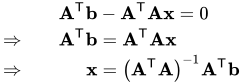
。 そこから並べ替えると
あ
T
b
−
あ
T
あ x
= 0
⇒
あ
T
b
=
あ
T
あ x
⇒
x
=
(
あ
T
あ
)
− 1
あ
T
b
{\displaystyle {\begin{aligned}&&\mathbf {A} ^{\textsf {T}}\mathbf {b} &-\mathbf {A} ^{\textsf {T}}\mathbf {Ax} =0 \\\Rightarrow &&\mathbf {A} ^{\textsf {T}}\mathbf {b} &=\mathbf {A} ^{\textsf {T}}\mathbf {Ax} \\\Rightarrow &&\mathbf {x} &=\left(\mathbf {A} ^{\textsf {T}}\mathbf {A} \right)^{-1} \mathbf {A} ^{\textsf {T}}\mathbf {b} \end{整列}}}
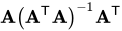
。 したがって、 は の列空間上にあるため、 に 写像する射影行列は です 。
あ x
{\displaystyle \mathbf {Ax} }
あ
{\displaystyle \mathbf {A} }
b
{\displaystyle \mathbf {b} }
x
{\displaystyle \mathbf {x} }
あ
(
あ
T
あ
)
− 1
あ
T
{\displaystyle \mathbf {A} \left(\mathbf {A} ^{\textsf {T}}\mathbf {A} \right)^{-1}\mathbf {A} ^{\textsf {T}} }
線形モデル 線形最小二乗法を使って線形モデルを推定したいとします。モデルは次のように記述できます。
ええ
=
バツ
β
+
ε
、
{\displaystyle \mathbf {y} =\mathbf {X} {\boldsymbol {\beta }}+{\boldsymbol {\varepsilon }},}
ここで、は 説明変数 の行列 ( 設計行列 )、 β は推定される未知のパラメータのベクトル、 ε は誤差ベクトルです。
バツ
{\displaystyle \mathbf {X} }
多くの種類のモデルと手法がこの定式化の対象となります。例としては、 線形最小二乗法 、 平滑化スプライン 、 回帰スプライン 、 局所回帰 、 カーネル回帰 、 線形フィルタリングなど があります。
通常の最小二乗法 各観測値の重みが同一で 誤差 が相関していない場合、推定パラメータは
β ^
=
(
バツ
T
バツ
)
− 1
バツ
T
ええ
、
{\displaystyle {\hat {\boldsymbol {\beta }}}=\left(\mathbf {X} ^{\textsf {T}}\mathbf {X} \right)^{-1}\mathbf {X} ^{\textsf {T}}\mathbf {y} ,}
したがって適合値は
ええ
^
=
バツ
β ^
=
バツ
(
バツ
T
バツ
)
− 1
バツ
T
ええ
。
{\displaystyle {\hat {\mathbf {y} }}=\mathbf {X} {\hat {\boldsymbol {\beta }}}=\mathbf {X} \left(\mathbf {X} ^{\textsf {T}}\mathbf {X} \right)^{-1}\mathbf {X} ^{\textsf {T}}\mathbf {y} .}
したがって、射影行列(およびハット行列)は次のように表される。
ポ
:=
バツ
(
バツ
T
バツ
)
− 1
バツ
T
。
{\displaystyle \mathbf {P} :=\mathbf {X} \left(\mathbf {X} ^{\textsf {T}}\mathbf {X} \right)^{-1}\mathbf {X} ^{\textsf {T}}.}
加重最小二乗法と一般化最小二乗法 上記は、重みが同一でない場合や誤差が相関している場合にも一般化できる。 誤差の 共分散行列が Σ であると仮定する。すると、
β
^
GLSA
=
(
バツ
T
Σ
− 1
バツ
)
− 1
バツ
T
Σ
− 1
ええ
{\displaystyle {\hat {\mathbf {\beta } }}_{\text{GLS}}=\left(\mathbf {X} ^{\textsf {T}}\mathbf {\Sigma } ^{-1}\mathbf {X} \right)^{-1}\mathbf {X} ^{\textsf {T}}\mathbf {\Sigma } ^{-1}\mathbf {y} }
。 帽子行列はこうなる
H
=
バツ
(
バツ
T
Σ
− 1
バツ
)
− 1
バツ
T
Σ
− 1
{\displaystyle \mathbf {H} =\mathbf {X} \left(\mathbf {X} ^{\textsf {T}}\mathbf {\Sigma } ^{-1}\mathbf {X} \right)^{-1}\mathbf {X} ^{\textsf {T}}\mathbf {\Sigma } ^{-1}}
そして再び であることが分かります が、今度は対称ではなくなりました。
H
2
= H ⋅ H = H
{\displaystyle H^{2}=H\cdot H=H}
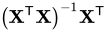
プロパティ 射影行列には、いくつかの有用な代数的性質がある。 [5] [6] 線型代数 の言語では 、射影行列は 計画行列の 列空間 への 直交射影 である。 [4] (は Xの擬似逆行列 である ことに注意してください 。)この設定での射影行列のいくつかの事実は、次のようにまとめられます。 [4]
X
{\displaystyle \mathbf {X} }
(
X
T
X
)
−
1
X
T
{\displaystyle \left(\mathbf {X} ^{\textsf {T}}\mathbf {X} \right)^{-1}\mathbf {X} ^{\textsf {T}}}
u
=
(
I
−
P
)
y
,
{\displaystyle \mathbf {u} =(\mathbf {I} -\mathbf {P} )\mathbf {y} ,}
そして
u
=
y
−
P
y
⊥
X
.
{\displaystyle \mathbf {u} =\mathbf {y} -\mathbf {P} \mathbf {y} \perp \mathbf {X} .}
P
{\displaystyle \mathbf {P} }
は対称であり、 も同様です 。
M
:=
I
−
P
{\displaystyle \mathbf {M} :=\mathbf {I} -\mathbf {P} }
P
{\displaystyle \mathbf {P} }
はべき等です: 、 も同様です 。
P
2
=
P
{\displaystyle \mathbf {P} ^{2}=\mathbf {P} }
M
{\displaystyle \mathbf {M} }
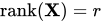
が n × r 行列で 、が成り立つ 場合、
X
{\displaystyle \mathbf {X} }
rank
(
X
)
=
r
{\displaystyle \operatorname {rank} (\mathbf {X} )=r}
rank
(
P
)
=
r
{\displaystyle \operatorname {rank} (\mathbf {P} )=r}
の 固有値 は r 個の1と n − r 個の0から構成され 、の固有値は n − r 個の1と r個 の0から構成されます 。 [7]
P
{\displaystyle \mathbf {P} }
M
{\displaystyle \mathbf {M} }
X
{\displaystyle \mathbf {X} }
は に関して不変です : したがって 。
P
{\displaystyle \mathbf {P} }
P
X
=
X
,
{\displaystyle \mathbf {PX} =\mathbf {X} ,}
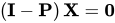
(
I
−
P
)
X
=
0
{\displaystyle \left(\mathbf {I} -\mathbf {P} \right)\mathbf {X} =\mathbf {0} }
(
I
−
P
)
P
=
P
(
I
−
P
)
=
0
.
{\displaystyle \left(\mathbf {I} -\mathbf {P} \right)\mathbf {P} =\mathbf {P} \left(\mathbf {I} -\mathbf {P} \right)=\mathbf {0} .}
P
{\displaystyle \mathbf {P} }
特定のサブスペースに対して一意です。 線形モデル に対応する投影行列は 対称 かつ べき等 です。 つまり、 です。ただし、常にそうであるとは限りません。たとえば、 局所加重散布図平滑化 (LOESS) では、ハット行列は一般に対称でもべき等でもありません。
P
2
=
P
{\displaystyle \mathbf {P} ^{2}=\mathbf {P} }
線型モデル の場合 、射影行列の トレース は の 階数 に等しく 、これは線型モデルの独立したパラメータの数です。 [8] 観測値において依然として線型であるLOESSなどの他のモデルの場合、射影行列を使用して モデルの
有効自由度を 定義できます。
X
{\displaystyle \mathbf {X} }
y
{\displaystyle \mathbf {y} }
回帰分析における投影行列の実際的な応用としては、 影響力のある観測値 、つまり回帰の結果に大きな影響を与える観測値
を特定することに関係するてこ 比 や クックの距離などがあります。
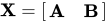
計画行列を 列ごとに と分解できるとします 。ハット演算子または射影演算子を と定義します 。同様に、残差演算子を と定義します 。すると、射影行列は次のように分解できます。 [9]
X
{\displaystyle \mathbf {X} }
X
=
[
A
B
]
{\displaystyle \mathbf {X} ={\begin{bmatrix}\mathbf {A} &\mathbf {B} \end{bmatrix}}}
P
[
X
]
:=
X
(
X
T
X
)
−
1
X
T
{\displaystyle \mathbf {P} [\mathbf {X} ]:=\mathbf {X} \left(\mathbf {X} ^{\textsf {T}}\mathbf {X} \right)^{-1}\mathbf {X} ^{\textsf {T}}}
M
[
X
]
:=
I
−
P
[
X
]
{\displaystyle \mathbf {M} [\mathbf {X} ]:=\mathbf {I} -\mathbf {P} [\mathbf {X} ]}
P
[
X
]
=
P
[
A
]
+
P
[
M
[
A
]
B
]
,
{\displaystyle \mathbf {P} [\mathbf {X} ]=\mathbf {P} [\mathbf {A} ]+\mathbf {P} {\big [}\mathbf {M} [\mathbf {A} ]\mathbf {B} {\big ]},}
ここで、例えば、 およびです 。このような分解には、さまざまな用途があります。古典的な用途では、 すべて 1 の列が使用され、これを使用して、回帰に切片項を追加した場合の効果を分析できます。もう 1 つの用途は、 固定効果モデル です。ここで、は固定効果項のダミー変数の 大きな 疎行列 です。この分割を使用すると、行列 を明示的に形成せずに、 のハット行列を計算できます 。行列 は大きすぎてコンピュータのメモリに収まらない場合があります。
P
[
A
]
=
A
(
A
T
A
)
−
1
A
T
{\displaystyle \mathbf {P} [\mathbf {A} ]=\mathbf {A} \left(\mathbf {A} ^{\textsf {T}}\mathbf {A} \right)^{-1}\mathbf {A} ^{\textsf {T}}}
M
[
A
]
=
I
−
P
[
A
]
{\displaystyle \mathbf {M} [\mathbf {A} ]=\mathbf {I} -\mathbf {P} [\mathbf {A} ]}
A
{\displaystyle \mathbf {A} }
A
{\displaystyle \mathbf {A} }
X
{\displaystyle \mathbf {X} }
X
{\displaystyle \mathbf {X} }
歴史 ハット行列は 1972 年に John Wilder によって導入されました。Hoaglin, DC と Welsch, RE (1978) による論文では、この行列の特性とその応用例が多数紹介されています。
参照
参考文献
^ Basilevsky, Alexander (2005). 統計科学における応用行列代数. Dover. pp. 160–176. ISBN 0-486-44538-0 。 ^ 「データ同化: データ同化システムの観測影響診断」 (PDF) 。2014年9月3日時点のオリジナル (PDF) からアーカイブ。 ^ ab Hoaglin, David C.; Welsch, Roy E. (1978年2月). 「回帰分析と分散分析におけるハット行列」 (PDF) . The American Statistician . 32 (1): 17–22. doi :10.2307/2683469. hdl : 1721.1/1920 . JSTOR 2683469. ^ abc David A. Freedman (2009). 統計モデル:理論と実践 . ケンブリッジ大学出版局 . ^ Gans, P. (1992). 化学科学におけるデータフィッティング . Wiley. ISBN 0-471-93412-7 。 ^ Draper, NR; Smith, H. (1998). 応用回帰分析 . Wiley. ISBN 0-471-17082-8 。 ^ 雨宮武 (1985). 上級計量経済学 . ケンブリッジ: ハーバード大学出版局. pp. 460–461. ISBN 0-674-00560-0 。 ^ 「線形回帰における「ハット」行列のトレースが X のランクであることの証明」 。Stack Exchange。2017 年 4 月 13 日。 ^ ラオ、C. ラダクリシュナ;トウテンブルク、ヘルゲ。シャラブ。ヒューマン、クリスチャン (2008)。 線形モデルと一般化 (第 3 版)。ベルリン:シュプリンガー。 p. 323.ISBN 978-3-540-74226-5 。




























![{\displaystyle \mathbf {P} [\mathbf {X} ]:=\mathbf {X} \left(\mathbf {X} ^{\textsf {T}}\mathbf {X} \right)^{-1}\mathbf {X} ^{\textsf {T}}}](https://wikimedia.org/api/rest_v1/media/math/render/svg/50598ad0872a5254026d7a5219ad04dedbc23fa2)
![{\displaystyle \mathbf {M} [\mathbf {X} ]:=\mathbf {I} -\mathbf {P} [\mathbf {X} ]}](https://wikimedia.org/api/rest_v1/media/math/render/svg/667297511e81442554a062b17f31cd9acdf16cda)
![{\displaystyle \mathbf {P} [\mathbf {X} ]=\mathbf {P} [\mathbf {A} ]+\mathbf {P} {\big [}\mathbf {M} [\mathbf {A} ]\mathbf {B} {\big ]},}](https://wikimedia.org/api/rest_v1/media/math/render/svg/99a9cbff4e154330b2e6ed410e1632416fc1393d)
![{\displaystyle \mathbf {P} [\mathbf {A} ]=\mathbf {A} \left(\mathbf {A} ^{\textsf {T}}\mathbf {A} \right)^{-1} \mathbf {A} ^{\textsf {T}}}](https://wikimedia.org/api/rest_v1/media/math/render/svg/a4fd598eeac379fe3ac02620d9eba5c41397df27)
![{\displaystyle \mathbf {M} [\mathbf {A} ]=\mathbf {I} -\mathbf {P} [\mathbf {A} ]}](https://wikimedia.org/api/rest_v1/media/math/render/svg/900711b6085ac5efe1486faf5239569052a0c229)