三角法 において 、 三角恒等式は 三角関数を 含む 等式 であり、 等式の両辺が定義されている発生 変数 のすべての値に対して真です。幾何学的には、これらは 1 つ以上の 角度の特定の関数を含む 恒等式です。これらは 三角形の恒等式 とは異なります。三角形の恒等式は、角度を含む可能性がある恒等式ですが、 三角形 の辺の長さやその他の長さも含みます 。
これらの恒等式は、三角関数を含む式を簡略化する必要がある場合に便利です。重要な応用例として、 非三角関数の 積分が挙げられます。一般的な手法としては、まず 三角関数で置換規則を 使用し、次に結果の積分を三角恒等式で簡略化します。
ピタゴラスの等式 三角関数と単位円上のその逆数。すべての直角三角形は相似です。つまり、対応する辺の比は同じです。sin、cos、tan の場合、単位長さの半径は、それらを定義する三角形の斜辺を形成します。逆数の恒等式は、この単位直線が斜辺ではなくなった三角形の辺の比として生じます。青色の三角形は恒等式 を示し 、赤色の三角形は を示しています 。
1 +
ベビーベッド
2
θ =
csc
2
θ
{\displaystyle 1+\cot^{2}\theta =\csc^{2}\theta }
日焼け
2
θ + 1 =
秒
2
θ
{\displaystyle \tan^{2}\theta +1=\sec^{2}\theta }
正弦と余弦 の基本的な関係は、 ピタゴラスの定理によって与えられます。
罪
2
θ +
コス
2
θ = 1 、
{\displaystyle \sin^{2}\theta +\cos^{2}\theta =1,}
ここで、 手段 と 手段
罪
2
θ
{\displaystyle \sin^{2}\theta }
( 罪 θ
)
2
{\displaystyle (\sin \theta )^{2}}
コス
2
θ
{\displaystyle \cos^{2}\theta }
( コス θ
)
2
。
{\displaystyle (\cos \theta )^{2}.}
これはピタゴラスの定理 の一種とみなすことができ 、 単位円 の方程式から導かれます 。この方程式は正弦または余弦のどちらについても解くことができます。
x
2
+
ええ
2
= 1
{\displaystyle x^{2}+y^{2}=1}
罪 θ
= ±
1 −
コス
2
θ
、
コス θ
= ±
1 −
罪
2
θ
。
{\displaystyle {\begin{aligned}\sin \theta &=\pm {\sqrt {1-\cos ^{2}\theta }},\\\cos \theta &=\pm {\sqrt {1- \sin ^{2}\theta }}.\end{整列}}}
ここで、符号は 象限 によって決まります
θ 。
{\displaystyle \theta .}
この恒等式を 、、 またはその両方で割ると、次の恒等式が得られます。
罪
2
θ
{\displaystyle \sin^{2}\theta }
コス
2
θ
{\displaystyle \cos^{2}\theta }
1 +
ベビーベッド
2
θ =
csc
2
θ
1 +
日焼け
2
θ =
秒
2
θ
秒
2
θ +
csc
2
θ =
秒
2
θ
csc
2
θ
{\displaystyle {\begin{aligned}&1+\cot ^{2}\theta =\csc ^{2}\theta \\&1+\tan ^{2}\theta =\sec ^{2}\theta \\&\sec ^{2}\theta +\csc ^{2}\theta =\sec ^{2}\theta \csc ^{2}\theta \end{aligned}}}
これらの恒等式を使用すると、任意の三角関数を他の任意の関数(プラスまたはマイナスの符号
まで )で表現できます。
反射、シフト、周期性 単位円を調べることによって、三角関数の次の特性を確立することができます。
反射 反射角 を1ずつシフトさせたときの座標( a 、 b )の変換
α
{\displaystyle \alpha }
π
4
{\displaystyle {\frac {\pi }{4}}}
ユークリッドベクトルの方向が角度で表される場合、 これは自由ベクトル(原点から始まる)と正の - 単位ベクトルによって決定される角度です。同じ概念はユークリッド空間の線にも適用できます。この場合、角度は原点と正の - 軸を通る指定された線に対する平行線によって決定されます。方向を持つ線(ベクトル)が 方向を持つ線について反射される場合 、この反射された線(ベクトル)の方向角は 値を持ちます。
θ
,
{\displaystyle \theta ,}
x
{\displaystyle x}
x
{\displaystyle x}
θ
{\displaystyle \theta }
α
,
{\displaystyle \alpha ,}
θ
′
{\displaystyle \theta ^{\prime }}
θ
′
=
2
α
−
θ
.
{\displaystyle \theta ^{\prime }=2\alpha -\theta .}
これらの角度の三角関数の特定の角度に対する 値は 、単純な恒等式を満たします。つまり、等しいか、反対の符号を持つか、相補三角関数を使用します。これらは 縮小公式 としても知られています。 [2]
θ
,
θ
′
{\displaystyle \theta ,\;\theta ^{\prime }}
α
{\displaystyle \alpha }
シフトと周期性 角度を 増分でシフトするときの 座標( a 、 b )の変換
θ
{\displaystyle \theta }
π
2
{\displaystyle {\frac {\pi }{2}}}
標識 三角関数の符号は角度の象限に依存する。sgn が 符号関数 で ある場合 、
−
π
<
θ
≤
π
{\displaystyle {-\pi }<\theta \leq \pi }
sgn
(
sin
θ
)
=
sgn
(
csc
θ
)
=
{
+
1
if
0
<
θ
<
π
−
1
if
−
π
<
θ
<
0
0
if
θ
∈
{
0
,
π
}
sgn
(
cos
θ
)
=
sgn
(
sec
θ
)
=
{
+
1
if
−
1
2
π
<
θ
<
1
2
π
−
1
if
−
π
<
θ
<
−
1
2
π
or
1
2
π
<
θ
<
π
0
if
θ
∈
{
−
1
2
π
,
1
2
π
}
sgn
(
tan
θ
)
=
sgn
(
cot
θ
)
=
{
+
1
if
−
π
<
θ
<
−
1
2
π
or
0
<
θ
<
1
2
π
−
1
if
−
1
2
π
<
θ
<
0
or
1
2
π
<
θ
<
π
0
if
θ
∈
{
−
1
2
π
,
0
,
1
2
π
,
π
}
{\displaystyle {\begin{aligned}\operatorname {sgn}(\sin \theta )=\operatorname {sgn}(\csc \theta )&={\begin{cases}+1&{\text{if}}\ \ 0<\theta <\pi \\-1&{\text{if}}\ \ {-\pi }<\theta <0\\0&{\text{if}}\ \ \theta \in \{0,\pi \}\end{cases}}\\[5mu]\operatorname {sgn}(\cos \theta )=\operatorname {sgn}(\sec \theta )&={\begin{cases}+1&{\text{if}}\ \ {-{\tfrac {1}{2}}\pi }<\theta <{\tfrac {1}{2}}\pi \\-1&{\text{if}}\ \ {-\pi }<\theta <-{\tfrac {1}{2}}\pi \ \ {\text{or}}\ \ {\tfrac {1}{2}}\pi <\theta <\pi \\0&{\text{if}}\ \ \theta \in {\bigl \{}{-{\tfrac {1}{2}}\pi },{\tfrac {1}{2}}\pi {\bigr \}}\end{cases}}\\[5mu]\operatorname {sgn}(\tan \theta )=\operatorname {sgn}(\cot \theta )&={\begin{cases}+1&{\text{if}}\ \ {-\pi }<\theta <-{\tfrac {1}{2}}\pi \ \ {\text{or}}\ \ 0<\theta <{\tfrac {1}{2}}\pi \\-1&{\text{if}}\ \ {-{\tfrac {1}{2}}\pi }<\theta <0\ \ {\text{or}}\ \ {\tfrac {1}{2}}\pi <\theta <\pi \\0&{\text{if}}\ \ \theta \in {\bigl \{}{-{\tfrac {1}{2}}\pi },0,{\tfrac {1}{2}}\pi ,\pi {\bigr \}}\end{cases}}\end{aligned}}}
三角関数は共通周期で周期的であるため、 区間外の θ の値については 繰り返し値を取ります (上記の § シフトと周期性を参照)。
2
π
,
{\displaystyle 2\pi ,}
(
−
π
,
π
]
,
{\displaystyle ({-\pi },\pi ],}
角度の和と差の等式 鋭角の正弦と余弦の角度の加算公式の図解。強調された線分は単位長さです。 および の角度差の恒等式を示す図
sin
(
α
−
β
)
{\displaystyle \sin(\alpha -\beta )}
cos
(
α
−
β
)
{\displaystyle \cos(\alpha -\beta )}
これらは角度の加減定理 (または 公式 )としても知られています 。
sin
(
α
+
β
)
=
sin
α
cos
β
+
cos
α
sin
β
sin
(
α
−
β
)
=
sin
α
cos
β
−
cos
α
sin
β
cos
(
α
+
β
)
=
cos
α
cos
β
−
sin
α
sin
β
cos
(
α
−
β
)
=
cos
α
cos
β
+
sin
α
sin
β
{\displaystyle {\begin{aligned}\sin(\alpha +\beta )&=\sin \alpha \cos \beta +\cos \alpha \sin \beta \\\sin(\alpha -\beta )&=\sin \alpha \cos \beta -\cos \alpha \sin \beta \\\cos(\alpha +\beta )&=\cos \alpha \cos \beta -\sin \alpha \sin \beta \\\cos(\alpha -\beta )&=\cos \alpha \cos \beta +\sin \alpha \sin \beta \end{aligned}}}
および の角度差恒等式は、 および という事実を使用 して、 を に代入して と と とを代入することで、角度和恒等式から 導くことができます。これらは、角度和恒等式の図をわずかに修正したものを使用して導くこともできます。ここでは、その両方を示します。
sin
(
α
−
β
)
{\displaystyle \sin(\alpha -\beta )}
cos
(
α
−
β
)
{\displaystyle \cos(\alpha -\beta )}
−
β
{\displaystyle -\beta }
β
{\displaystyle \beta }
sin
(
−
β
)
=
−
sin
(
β
)
{\displaystyle \sin(-\beta )=-\sin(\beta )}
cos
(
−
β
)
=
cos
(
β
)
{\displaystyle \cos(-\beta )=\cos(\beta )}
これらの恒等式は次の表の最初の 2 行にまとめられています。この表には、他の三角関数の和恒等式と差恒等式も含まれています。
無限の角度の和の正弦と余弦 級数が 絶対収束する と
∑
i
=
1
∞
θ
i
{\textstyle \sum _{i=1}^{\infty }\theta _{i}}
sin
(
∑
i
=
1
∞
θ
i
)
=
∑
odd
k
≥
1
(
−
1
)
k
−
1
2
∑
A
⊆
{
1
,
2
,
3
,
…
}
|
A
|
=
k
(
∏
i
∈
A
sin
θ
i
∏
i
∉
A
cos
θ
i
)
cos
(
∑
i
=
1
∞
θ
i
)
=
∑
even
k
≥
0
(
−
1
)
k
2
∑
A
⊆
{
1
,
2
,
3
,
…
}
|
A
|
=
k
(
∏
i
∈
A
sin
θ
i
∏
i
∉
A
cos
θ
i
)
.
{\displaystyle {\begin{aligned}{\sin }{\biggl (}\sum _{i=1}^{\infty }\theta _{i}{\biggl )}&=\sum _{{\text{odd}}\ k\geq 1}(-1)^{\frac {k-1}{2}}\!\!\sum _{\begin{smallmatrix}A\subseteq \{\,1,2,3,\dots \,\}\\\left|A\right|=k\end{smallmatrix}}{\biggl (}\prod _{i\in A}\sin \theta _{i}\prod _{i\not \in A}\cos \theta _{i}{\biggr )}\\{\cos }{\biggl (}\sum _{i=1}^{\infty }\theta _{i}{\biggr )}&=\sum _{{\text{even}}\ k\geq 0}(-1)^{\frac {k}{2}}\,\sum _{\begin{smallmatrix}A\subseteq \{\,1,2,3,\dots \,\}\\\left|A\right|=k\end{smallmatrix}}{\biggl (}\prod _{i\in A}\sin \theta _{i}\prod _{i\not \in A}\cos \theta _{i}{\biggr )}.\end{aligned}}}
この級数は 絶対収束するので、必然的に かつ となります 。特に、これら 2 つの恒等式では、有限個の角度の和の場合には見られない非対称性が現れます。つまり、各積において、正弦因子は有限個しかありませんが、余弦因子は余有限個あります 。 正弦 因子が無限個ある項は必然的に 0 になります。
∑
i
=
1
∞
θ
i
{\textstyle \sum _{i=1}^{\infty }\theta _{i}}
lim
i
→
∞
θ
i
=
0
,
{\textstyle \lim _{i\to \infty }\theta _{i}=0,}
lim
i
→
∞
sin
θ
i
=
0
,
{\textstyle \lim _{i\to \infty }\sin \theta _{i}=0,}
lim
i
→
∞
cos
θ
i
=
1.
{\textstyle \lim _{i\to \infty }\cos \theta _{i}=1.}
角度のうち、有限個のみ が非ゼロである場合、右側の項のうち、有限個のみが非ゼロになります。これは、正弦係数のうち有限個以外はすべて消えるためです。さらに、各項において、余弦係数のうち有限個以外はすべて 1 です。
θ
i
{\displaystyle \theta _{i}}
和の正接と余接 (に対して )を 変数の
k 次 基本対称多項式 とする
と 、
e
k
{\displaystyle e_{k}}
k
=
0
,
1
,
2
,
3
,
…
{\displaystyle k=0,1,2,3,\ldots }
x
i
=
tan
θ
i
{\displaystyle x_{i}=\tan \theta _{i}}
i
=
0
,
1
,
2
,
3
,
…
,
{\displaystyle i=0,1,2,3,\ldots ,}
e
0
=
1
e
1
=
∑
i
x
i
=
∑
i
tan
θ
i
e
2
=
∑
i
<
j
x
i
x
j
=
∑
i
<
j
tan
θ
i
tan
θ
j
e
3
=
∑
i
<
j
<
k
x
i
x
j
x
k
=
∑
i
<
j
<
k
tan
θ
i
tan
θ
j
tan
θ
k
⋮
⋮
{\displaystyle {\begin{aligned}e_{0}&=1\\[6pt]e_{1}&=\sum _{i}x_{i}&&=\sum _{i}\tan \theta _{i}\\[6pt]e_{2}&=\sum _{i<j}x_{i}x_{j}&&=\sum _{i<j}\tan \theta _{i}\tan \theta _{j}\\[6pt]e_{3}&=\sum _{i<j<k}x_{i}x_{j}x_{k}&&=\sum _{i<j<k}\tan \theta _{i}\tan \theta _{j}\tan \theta _{k}\\&\ \ \vdots &&\ \ \vdots \end{aligned}}}
それから
tan
(
∑
i
θ
i
)
=
sin
(
∑
i
θ
i
)
/
∏
i
cos
θ
i
cos
(
∑
i
θ
i
)
/
∏
i
cos
θ
i
=
∑
odd
k
≥
1
(
−
1
)
k
−
1
2
∑
A
⊆
{
1
,
2
,
3
,
…
}
|
A
|
=
k
∏
i
∈
A
tan
θ
i
∑
even
k
≥
0
(
−
1
)
k
2
∑
A
⊆
{
1
,
2
,
3
,
…
}
|
A
|
=
k
∏
i
∈
A
tan
θ
i
=
e
1
−
e
3
+
e
5
−
⋯
e
0
−
e
2
+
e
4
−
⋯
cot
(
∑
i
θ
i
)
=
e
0
−
e
2
+
e
4
−
⋯
e
1
−
e
3
+
e
5
−
⋯
{\displaystyle {\begin{aligned}{\tan }{\Bigl (}\sum _{i}\theta _{i}{\Bigr )}&={\frac {{\sin }{\bigl (}\sum _{i}\theta _{i}{\bigr )}/\prod _{i}\cos \theta _{i}}{{\cos }{\bigl (}\sum _{i}\theta _{i}{\bigr )}/\prod _{i}\cos \theta _{i}}}\\[10pt]&={\frac {\displaystyle \sum _{{\text{odd}}\ k\geq 1}(-1)^{\frac {k-1}{2}}\sum _{\begin{smallmatrix}A\subseteq \{1,2,3,\dots \}\\\left|A\right|=k\end{smallmatrix}}\prod _{i\in A}\tan \theta _{i}}{\displaystyle \sum _{{\text{even}}\ k\geq 0}~(-1)^{\frac {k}{2}}~~\sum _{\begin{smallmatrix}A\subseteq \{1,2,3,\dots \}\\\left|A\right|=k\end{smallmatrix}}\prod _{i\in A}\tan \theta _{i}}}={\frac {e_{1}-e_{3}+e_{5}-\cdots }{e_{0}-e_{2}+e_{4}-\cdots }}\\[10pt]{\cot }{\Bigl (}\sum _{i}\theta _{i}{\Bigr )}&={\frac {e_{0}-e_{2}+e_{4}-\cdots }{e_{1}-e_{3}+e_{5}-\cdots }}\end{aligned}}}
上記の正弦と余弦の合計の公式を使用します。
右側の項の数は左側の項の数によって決まります。
例えば:
tan
(
θ
1
+
θ
2
)
=
e
1
e
0
−
e
2
=
x
1
+
x
2
1
−
x
1
x
2
=
tan
θ
1
+
tan
θ
2
1
−
tan
θ
1
tan
θ
2
,
tan
(
θ
1
+
θ
2
+
θ
3
)
=
e
1
−
e
3
e
0
−
e
2
=
(
x
1
+
x
2
+
x
3
)
−
(
x
1
x
2
x
3
)
1
−
(
x
1
x
2
+
x
1
x
3
+
x
2
x
3
)
,
tan
(
θ
1
+
θ
2
+
θ
3
+
θ
4
)
=
e
1
−
e
3
e
0
−
e
2
+
e
4
=
(
x
1
+
x
2
+
x
3
+
x
4
)
−
(
x
1
x
2
x
3
+
x
1
x
2
x
4
+
x
1
x
3
x
4
+
x
2
x
3
x
4
)
1
−
(
x
1
x
2
+
x
1
x
3
+
x
1
x
4
+
x
2
x
3
+
x
2
x
4
+
x
3
x
4
)
+
(
x
1
x
2
x
3
x
4
)
,
{\displaystyle {\begin{aligned}\tan(\theta _{1}+\theta _{2})&={\frac {e_{1}}{e_{0}-e_{2}}}={\frac {x_{1}+x_{2}}{1\ -\ x_{1}x_{2}}}={\frac {\tan \theta _{1}+\tan \theta _{2}}{1\ -\ \tan \theta _{1}\tan \theta _{2}}},\\[8pt]\tan(\theta _{1}+\theta _{2}+\theta _{3})&={\frac {e_{1}-e_{3}}{e_{0}-e_{2}}}={\frac {(x_{1}+x_{2}+x_{3})\ -\ (x_{1}x_{2}x_{3})}{1\ -\ (x_{1}x_{2}+x_{1}x_{3}+x_{2}x_{3})}},\\[8pt]\tan(\theta _{1}+\theta _{2}+\theta _{3}+\theta _{4})&={\frac {e_{1}-e_{3}}{e_{0}-e_{2}+e_{4}}}\\[8pt]&={\frac {(x_{1}+x_{2}+x_{3}+x_{4})\ -\ (x_{1}x_{2}x_{3}+x_{1}x_{2}x_{4}+x_{1}x_{3}x_{4}+x_{2}x_{3}x_{4})}{1\ -\ (x_{1}x_{2}+x_{1}x_{3}+x_{1}x_{4}+x_{2}x_{3}+x_{2}x_{4}+x_{3}x_{4})\ +\ (x_{1}x_{2}x_{3}x_{4})}},\end{aligned}}}
などなど。項が有限個の場合は 数学的帰納法 で証明できる。 [14] 項が無限個の場合はいくつかの基本的な不等式を使って証明できる。 [15]
和の割線と余割線
sec
(
∑
i
θ
i
)
=
∏
i
sec
θ
i
e
0
−
e
2
+
e
4
−
⋯
csc
(
∑
i
θ
i
)
=
∏
i
sec
θ
i
e
1
−
e
3
+
e
5
−
⋯
{\displaystyle {\begin{aligned}{\sec }{\Bigl (}\sum _{i}\theta _{i}{\Bigr )}&={\frac {\prod _{i}\sec \theta _{i}}{e_{0}-e_{2}+e_{4}-\cdots }}\\[8pt]{\csc }{\Bigl (}\sum _{i}\theta _{i}{\Bigr )}&={\frac {\prod _{i}\sec \theta _{i}}{e_{1}-e_{3}+e_{5}-\cdots }}\end{aligned}}}
ここで、は n 変数 の k 次 基本対称多項式 であり 、分母の項の数と分子の積の因数の数は、左側の和の項の数に依存します。 [16] 項が有限個の場合は、そのような項の数に関する数学的帰納法によって証明できます。
e
k
{\displaystyle e_{k}}
x
i
=
tan
θ
i
,
{\displaystyle x_{i}=\tan \theta _{i},}
i
=
1
,
…
,
n
,
{\displaystyle i=1,\ldots ,n,}
例えば、
sec
(
α
+
β
+
γ
)
=
sec
α
sec
β
sec
γ
1
−
tan
α
tan
β
−
tan
α
tan
γ
−
tan
β
tan
γ
csc
(
α
+
β
+
γ
)
=
sec
α
sec
β
sec
γ
tan
α
+
tan
β
+
tan
γ
−
tan
α
tan
β
tan
γ
.
{\displaystyle {\begin{aligned}\sec(\alpha +\beta +\gamma )&={\frac {\sec \alpha \sec \beta \sec \gamma }{1-\tan \alpha \tan \beta -\tan \alpha \tan \gamma -\tan \beta \tan \gamma }}\\[8pt]\csc(\alpha +\beta +\gamma )&={\frac {\sec \alpha \sec \beta \sec \gamma }{\tan \alpha +\tan \beta +\tan \gamma -\tan \alpha \tan \beta \tan \gamma }}.\end{aligned}}}
プトレマイオスの定理 プトレマイオスの定理と正弦の角度の和の三角恒等式の関係を示す図。プトレマイオスの定理は、対辺の長さの積の合計が対角線の長さの積に等しいと述べています。これらの辺の長さを、上の図に示されている sin 値と cos 値で表すと、正弦の角度の和の三角恒等式 sin( α + β ) = sin α cos β + cos α sin β が得られます。 プトレマイオスの定理は三角関数の恒等式の歴史において重要な定理である。これは、正弦と余弦の和と差の公式と同等の結果が初めて証明された方法だからである。それは、 図に示すように、円周四辺形において、対辺の長さの積の和は対角線の長さの積に等しいことを述べている。対角線または辺の1つが円の直径である特殊なケースでは、この定理から角度の和と差の三角関数の恒等式が直接導かれる。 [17] ここに示すように、円の直径が長さ1になるように作図すると、関係が最も簡単にわかる。
A
B
C
D
{\displaystyle ABCD}
タレスの定理 によれば 、、 およびは ともに直角です。直角三角形 および は ともに長さ 1 の斜辺を共有しています。 したがって、辺 、 、 および です 。
∠
D
A
B
{\displaystyle \angle DAB}
∠
D
C
B
{\displaystyle \angle DCB}
D
A
B
{\displaystyle DAB}
D
C
B
{\displaystyle DCB}
B
D
¯
{\displaystyle {\overline {BD}}}
A
B
¯
=
sin
α
{\displaystyle {\overline {AB}}=\sin \alpha }
A
D
¯
=
cos
α
{\displaystyle {\overline {AD}}=\cos \alpha }
B
C
¯
=
sin
β
{\displaystyle {\overline {BC}}=\sin \beta }
C
D
¯
=
cos
β
{\displaystyle {\overline {CD}}=\cos \beta }
円周角の 定理により、 円の中心の 弦によって囲まれる中心角は、角度 の 2 倍 、つまり です 。したがって、対称的な 1 組の赤い三角形はそれぞれ、 中心に角度 を持ちます。これらの三角形の斜辺の長さはそれぞれ である ため、 の長さは 、 つまり単に です 。四辺形のもう 1 つの対角線は直径で長さ 1 であるため、対角線の長さの積も です 。
A
C
¯
{\displaystyle {\overline {AC}}}
∠
A
D
C
{\displaystyle \angle ADC}
2
(
α
+
β
)
{\displaystyle 2(\alpha +\beta )}
α
+
β
{\displaystyle \alpha +\beta }
1
2
{\textstyle {\frac {1}{2}}}
A
C
¯
{\displaystyle {\overline {AC}}}
2
×
1
2
sin
(
α
+
β
)
{\textstyle 2\times {\frac {1}{2}}\sin(\alpha +\beta )}
sin
(
α
+
β
)
{\displaystyle \sin(\alpha +\beta )}
sin
(
α
+
β
)
{\displaystyle \sin(\alpha +\beta )}
これらの値をプトレマイオスの定理の に代入すると 、正弦の角度の和の三角関数恒等式が得られます。 の角度差の公式は、 の代わりに を直径として 同様に導くことができます 。 [17]
|
A
C
¯
|
⋅
|
B
D
¯
|
=
|
A
B
¯
|
⋅
|
C
D
¯
|
+
|
A
D
¯
|
⋅
|
B
C
¯
|
{\displaystyle |{\overline {AC}}|\cdot |{\overline {BD}}|=|{\overline {AB}}|\cdot |{\overline {CD}}|+|{\overline {AD}}|\cdot |{\overline {BC}}|}
sin
(
α
+
β
)
=
sin
α
cos
β
+
cos
α
sin
β
{\displaystyle \sin(\alpha +\beta )=\sin \alpha \cos \beta +\cos \alpha \sin \beta }
sin
(
α
−
β
)
{\displaystyle \sin(\alpha -\beta )}
C
D
¯
{\displaystyle {\overline {CD}}}
B
D
¯
{\displaystyle {\overline {BD}}}
正弦の二倍角の公式の視覚的な説明。上記の単位辺と角度を持つ二等辺三角形の 面積は
2
θ
{\displaystyle 2\theta }
1 / 2 × 底辺 × 高さは2つの方向で計算されます。直立しているとき、面積は です 。横になっているとき、同じ面積は です 。したがって、
sin
θ
cos
θ
{\displaystyle \sin \theta \cos \theta }
1
2
sin
2
θ
{\textstyle {\frac {1}{2}}\sin 2\theta }
sin
2
θ
=
2
sin
θ
cos
θ
.
{\displaystyle \sin 2\theta =2\sin \theta \cos \theta .}
角度の2倍の公式。 [20]
sin
(
2
θ
)
=
2
sin
θ
cos
θ
=
(
sin
θ
+
cos
θ
)
2
−
1
=
2
tan
θ
1
+
tan
2
θ
{\displaystyle \sin(2\theta )=2\sin \theta \cos \theta =(\sin \theta +\cos \theta )^{2}-1={\frac {2\tan \theta }{1+\tan ^{2}\theta }}}
cos
(
2
θ
)
=
cos
2
θ
−
sin
2
θ
=
2
cos
2
θ
−
1
=
1
−
2
sin
2
θ
=
1
−
tan
2
θ
1
+
tan
2
θ
{\displaystyle \cos(2\theta )=\cos ^{2}\theta -\sin ^{2}\theta =2\cos ^{2}\theta -1=1-2\sin ^{2}\theta ={\frac {1-\tan ^{2}\theta }{1+\tan ^{2}\theta }}}
tan
(
2
θ
)
=
2
tan
θ
1
−
tan
2
θ
{\displaystyle \tan(2\theta )={\frac {2\tan \theta }{1-\tan ^{2}\theta }}}
cot
(
2
θ
)
=
cot
2
θ
−
1
2
cot
θ
=
1
−
tan
2
θ
2
tan
θ
{\displaystyle \cot(2\theta )={\frac {\cot ^{2}\theta -1}{2\cot \theta }}={\frac {1-\tan ^{2}\theta }{2\tan \theta }}}
sec
(
2
θ
)
=
sec
2
θ
2
−
sec
2
θ
=
1
+
tan
2
θ
1
−
tan
2
θ
{\displaystyle \sec(2\theta )={\frac {\sec ^{2}\theta }{2-\sec ^{2}\theta }}={\frac {1+\tan ^{2}\theta }{1-\tan ^{2}\theta }}}
csc
(
2
θ
)
=
sec
θ
csc
θ
2
=
1
+
tan
2
θ
2
tan
θ
{\displaystyle \csc(2\theta )={\frac {\sec \theta \csc \theta }{2}}={\frac {1+\tan ^{2}\theta }{2\tan \theta }}}
三角角の公式。 [20]
sin
(
3
θ
)
=
3
sin
θ
−
4
sin
3
θ
=
4
sin
θ
sin
(
π
3
−
θ
)
sin
(
π
3
+
θ
)
{\displaystyle \sin(3\theta )=3\sin \theta -4\sin ^{3}\theta =4\sin \theta \sin \left({\frac {\pi }{3}}-\theta \right)\sin \left({\frac {\pi }{3}}+\theta \right)}
cos
(
3
θ
)
=
4
cos
3
θ
−
3
cos
θ
=
4
cos
θ
cos
(
π
3
−
θ
)
cos
(
π
3
+
θ
)
{\displaystyle \cos(3\theta )=4\cos ^{3}\theta -3\cos \theta =4\cos \theta \cos \left({\frac {\pi }{3}}-\theta \right)\cos \left({\frac {\pi }{3}}+\theta \right)}
tan
(
3
θ
)
=
3
tan
θ
−
tan
3
θ
1
−
3
tan
2
θ
=
tan
θ
tan
(
π
3
−
θ
)
tan
(
π
3
+
θ
)
{\displaystyle \tan(3\theta )={\frac {3\tan \theta -\tan ^{3}\theta }{1-3\tan ^{2}\theta }}=\tan \theta \tan \left({\frac {\pi }{3}}-\theta \right)\tan \left({\frac {\pi }{3}}+\theta \right)}
cot
(
3
θ
)
=
3
cot
θ
−
cot
3
θ
1
−
3
cot
2
θ
{\displaystyle \cot(3\theta )={\frac {3\cot \theta -\cot ^{3}\theta }{1-3\cot ^{2}\theta }}}
sec
(
3
θ
)
=
sec
3
θ
4
−
3
sec
2
θ
{\displaystyle \sec(3\theta )={\frac {\sec ^{3}\theta }{4-3\sec ^{2}\theta }}}
csc
(
3
θ
)
=
csc
3
θ
3
csc
2
θ
−
4
{\displaystyle \csc(3\theta )={\frac {\csc ^{3}\theta }{3\csc ^{2}\theta -4}}}
多重角度の公式。 [21]
sin
(
n
θ
)
=
∑
k
odd
(
−
1
)
k
−
1
2
(
n
k
)
cos
n
−
k
θ
sin
k
θ
=
sin
θ
∑
i
=
0
(
n
+
1
)
/
2
∑
j
=
0
i
(
−
1
)
i
−
j
(
n
2
i
+
1
)
(
i
j
)
cos
n
−
2
(
i
−
j
)
−
1
θ
=
sin
(
θ
)
⋅
∑
k
=
0
⌊
n
−
1
2
⌋
(
−
1
)
k
⋅
(
2
⋅
cos
(
θ
)
)
n
−
2
k
−
1
⋅
(
n
−
k
−
1
k
)
=
2
(
n
−
1
)
∏
k
=
0
n
−
1
sin
(
k
π
/
n
+
θ
)
{\displaystyle {\begin{aligned}\sin(n\theta )&=\sum _{k{\text{ odd}}}(-1)^{\frac {k-1}{2}}{n \choose k}\cos ^{n-k}\theta \sin ^{k}\theta =\sin \theta \sum _{i=0}^{(n+1)/2}\sum _{j=0}^{i}(-1)^{i-j}{n \choose 2i+1}{i \choose j}\cos ^{n-2(i-j)-1}\theta \\{}&=\sin(\theta )\cdot \sum _{k=0}^{\left\lfloor {\frac {n-1}{2}}\right\rfloor }(-1)^{k}\cdot {(2\cdot \cos(\theta ))}^{n-2k-1}\cdot {n-k-1 \choose k}\\{}&=2^{(n-1)}\prod _{k=0}^{n-1}\sin(k\pi /n+\theta )\end{aligned}}}
cos
(
n
θ
)
=
∑
k
even
(
−
1
)
k
2
(
n
k
)
cos
n
−
k
θ
sin
k
θ
=
∑
i
=
0
n
/
2
∑
j
=
0
i
(
−
1
)
i
−
j
(
n
2
i
)
(
i
j
)
cos
n
−
2
(
i
−
j
)
θ
=
∑
k
=
0
⌊
n
2
⌋
(
−
1
)
k
⋅
(
2
⋅
cos
(
θ
)
)
n
−
2
k
⋅
(
n
−
k
k
)
⋅
n
2
n
−
2
k
{\displaystyle {\begin{aligned}\cos(n\theta )&=\sum _{k{\text{ even}}}(-1)^{\frac {k}{2}}{n \choose k}\cos ^{n-k}\theta \sin ^{k}\theta =\sum _{i=0}^{n/2}\sum _{j=0}^{i}(-1)^{i-j}{n \choose 2i}{i \choose j}\cos ^{n-2(i-j)}\theta \\{}&=\sum _{k=0}^{\left\lfloor {\frac {n}{2}}\right\rfloor }(-1)^{k}\cdot {(2\cdot \cos(\theta ))}^{n-2k}\cdot {n-k \choose k}\cdot {\frac {n}{2n-2k}}\end{aligned}}}
cos
(
(
2
n
+
1
)
θ
)
=
(
−
1
)
n
2
2
n
∏
k
=
0
2
n
cos
(
k
π
/
(
2
n
+
1
)
−
θ
)
{\displaystyle \cos((2n+1)\theta )=(-1)^{n}2^{2n}\prod _{k=0}^{2n}\cos(k\pi /(2n+1)-\theta )}
cos
(
2
n
θ
)
=
(
−
1
)
n
2
2
n
−
1
∏
k
=
0
2
n
−
1
cos
(
(
1
+
2
k
)
π
/
(
4
n
)
−
θ
)
{\displaystyle \cos(2n\theta )=(-1)^{n}2^{2n-1}\prod _{k=0}^{2n-1}\cos((1+2k)\pi /(4n)-\theta )}
tan
(
n
θ
)
=
∑
k
odd
(
−
1
)
k
−
1
2
(
n
k
)
tan
k
θ
∑
k
even
(
−
1
)
k
2
(
n
k
)
tan
k
θ
{\displaystyle \tan(n\theta )={\frac {\sum _{k{\text{ odd}}}(-1)^{\frac {k-1}{2}}{n \choose k}\tan ^{k}\theta }{\sum _{k{\text{ even}}}(-1)^{\frac {k}{2}}{n \choose k}\tan ^{k}\theta }}}
チェビシェフ法 チェビシェフ法は 、 番目と番目の値がわかっている場合に n 番目の倍数角度の式 を見つけるための 再帰 アルゴリズム です 。 [22]
(
n
−
1
)
{\displaystyle (n-1)}
(
n
−
2
)
{\displaystyle (n-2)}
cos
(
n
x
)
{\displaystyle \cos(nx)}
は
、、、 および から計算でき、
cos
(
(
n
−
1
)
x
)
{\displaystyle \cos((n-1)x)}
cos
(
(
n
−
2
)
x
)
{\displaystyle \cos((n-2)x)}
cos
(
x
)
{\displaystyle \cos(x)}
cos
(
n
x
)
=
2
cos
x
cos
(
(
n
−
1
)
x
)
−
cos
(
(
n
−
2
)
x
)
.
{\displaystyle \cos(nx)=2\cos x\cos((n-1)x)-\cos((n-2)x).}
これは、次の式を足し合わせることで証明できる。
cos
(
(
n
−
1
)
x
+
x
)
=
cos
(
(
n
−
1
)
x
)
cos
x
−
sin
(
(
n
−
1
)
x
)
sin
x
cos
(
(
n
−
1
)
x
−
x
)
=
cos
(
(
n
−
1
)
x
)
cos
x
+
sin
(
(
n
−
1
)
x
)
sin
x
{\displaystyle {\begin{aligned}\cos((n-1)x+x)&=\cos((n-1)x)\cos x-\sin((n-1)x)\sin x\\\cos((n-1)x-x)&=\cos((n-1)x)\cos x+\sin((n-1)x)\sin x\end{aligned}}}
帰納的に、 は いわゆる第一種チェビシェフ多項式 の多項式であることがわかります。 チェビシェフ多項式#三角関数の定義 を参照してください。
cos
(
n
x
)
{\displaystyle \cos(nx)}
cos
x
,
{\displaystyle \cos x,}
同様に、は、 およびから 計算できます 。
これは、 および
の公式を追加することで証明できます。
sin
(
n
x
)
{\displaystyle \sin(nx)}
sin
(
(
n
−
1
)
x
)
,
{\displaystyle \sin((n-1)x),}
sin
(
(
n
−
2
)
x
)
,
{\displaystyle \sin((n-2)x),}
cos
x
{\displaystyle \cos x}
sin
(
n
x
)
=
2
cos
x
sin
(
(
n
−
1
)
x
)
−
sin
(
(
n
−
2
)
x
)
{\displaystyle \sin(nx)=2\cos x\sin((n-1)x)-\sin((n-2)x)}
sin
(
(
n
−
1
)
x
+
x
)
{\displaystyle \sin((n-1)x+x)}
sin
(
(
n
−
1
)
x
−
x
)
.
{\displaystyle \sin((n-1)x-x).}
チェビシェフ法と同様の目的を果たす接線については、次のように記述できます。
tan
(
n
x
)
=
tan
(
(
n
−
1
)
x
)
+
tan
x
1
−
tan
(
(
n
−
1
)
x
)
tan
x
.
{\displaystyle \tan(nx)={\frac {\tan((n-1)x)+\tan x}{1-\tan((n-1)x)\tan x}}\,.}
sin
θ
2
=
sgn
(
sin
θ
2
)
1
−
cos
θ
2
cos
θ
2
=
sgn
(
cos
θ
2
)
1
+
cos
θ
2
tan
θ
2
=
1
−
cos
θ
sin
θ
=
sin
θ
1
+
cos
θ
=
csc
θ
−
cot
θ
=
tan
θ
1
+
sec
θ
=
sgn
(
sin
θ
)
1
−
cos
θ
1
+
cos
θ
=
−
1
+
sgn
(
cos
θ
)
1
+
tan
2
θ
tan
θ
cot
θ
2
=
1
+
cos
θ
sin
θ
=
sin
θ
1
−
cos
θ
=
csc
θ
+
cot
θ
=
sgn
(
sin
θ
)
1
+
cos
θ
1
−
cos
θ
sec
θ
2
=
sgn
(
cos
θ
2
)
2
1
+
cos
θ
csc
θ
2
=
sgn
(
sin
θ
2
)
2
1
−
cos
θ
{\displaystyle {\begin{aligned}\sin {\frac {\theta }{2}}&=\operatorname {sgn} \left(\sin {\frac {\theta }{2}}\right){\sqrt {\frac {1-\cos \theta }{2}}}\\[3pt]\cos {\frac {\theta }{2}}&=\operatorname {sgn} \left(\cos {\frac {\theta }{2}}\right){\sqrt {\frac {1+\cos \theta }{2}}}\\[3pt]\tan {\frac {\theta }{2}}&={\frac {1-\cos \theta }{\sin \theta }}={\frac {\sin \theta }{1+\cos \theta }}=\csc \theta -\cot \theta ={\frac {\tan \theta }{1+\sec {\theta }}}\\[6mu]&=\operatorname {sgn}(\sin \theta ){\sqrt {\frac {1-\cos \theta }{1+\cos \theta }}}={\frac {-1+\operatorname {sgn}(\cos \theta ){\sqrt {1+\tan ^{2}\theta }}}{\tan \theta }}\\[3pt]\cot {\frac {\theta }{2}}&={\frac {1+\cos \theta }{\sin \theta }}={\frac {\sin \theta }{1-\cos \theta }}=\csc \theta +\cot \theta =\operatorname {sgn}(\sin \theta ){\sqrt {\frac {1+\cos \theta }{1-\cos \theta }}}\\\sec {\frac {\theta }{2}}&=\operatorname {sgn} \left(\cos {\frac {\theta }{2}}\right){\sqrt {\frac {2}{1+\cos \theta }}}\\\csc {\frac {\theta }{2}}&=\operatorname {sgn} \left(\sin {\frac {\theta }{2}}\right){\sqrt {\frac {2}{1-\cos \theta }}}\\\end{aligned}}}
[23] [24]
また
tan
η
±
θ
2
=
sin
η
±
sin
θ
cos
η
+
cos
θ
tan
(
θ
2
+
π
4
)
=
sec
θ
+
tan
θ
1
−
sin
θ
1
+
sin
θ
=
|
1
−
tan
θ
2
|
|
1
+
tan
θ
2
|
{\displaystyle {\begin{aligned}\tan {\frac {\eta \pm \theta }{2}}&={\frac {\sin \eta \pm \sin \theta }{\cos \eta +\cos \theta }}\\[3pt]\tan \left({\frac {\theta }{2}}+{\frac {\pi }{4}}\right)&=\sec \theta +\tan \theta \\[3pt]{\sqrt {\frac {1-\sin \theta }{1+\sin \theta }}}&={\frac {\left|1-\tan {\frac {\theta }{2}}\right|}{\left|1+\tan {\frac {\theta }{2}}\right|}}\end{aligned}}}
テーブル これらは、和と差の恒等式、または倍数角度の公式のいずれかを使用して表示できます。
正弦と余弦の三重角の公式には単一の関数の累乗しか含まれていないという事実により、 コンパスと定規を使用して 角 の三等分を作成するという幾何学の問題を、 三次方程式 を解くという代数の問題に関連付けることができます。これにより、与えられたツールを使用した 三等分は一般に不可能であること を証明できます 。
1/3 角の三角恒等式を計算する公式は存在しますが、 3 次方程式 4 x 3 − 3 x + d = 0 の零点を見つける必要があります。ここで、 は 1/3 角における余弦関数の値、 d は 全角における余弦関数の既知の値です。ただし、この方程式の 判別式 は正であるため、この方程式には 3 つの実根があります (そのうち 1 つだけが 1/3 角の余弦の解です)。これらの解はいずれも、 3 次根 の下で中間の複素数を使用するため、 実 数式に 還元できません 。
x
{\displaystyle x}
余弦二倍角の公式の 2 番目と 3 番目のバージョンを解くことによって得られます。
コサインのべき乗減少式: 説明図。赤、オレンジ、青の三角形はすべて相似で、赤とオレンジの三角形は合同です。 青の三角形の斜辺の長さは です 。角度 は なので 、その三角形の底辺 の長さは です。その長さは、 と の長さの合計にも等しく 、つまり です 。したがって、 です。 両辺を で割ると、 コサインのべき乗減少式が得られます。 。コサインの半角の式は、 を に置き換え て両辺の平方根を取ることで得られます。
A
D
¯
{\displaystyle {\overline {AD}}}
2
cos
θ
{\displaystyle 2\cos \theta }
∠
D
A
E
{\displaystyle \angle DAE}
θ
{\displaystyle \theta }
A
E
¯
{\displaystyle {\overline {AE}}}
2
cos
2
θ
{\displaystyle 2\cos ^{2}\theta }
B
D
¯
{\displaystyle {\overline {BD}}}
A
F
¯
{\displaystyle {\overline {AF}}}
1
+
cos
(
2
θ
)
{\displaystyle 1+\cos(2\theta )}
2
cos
2
θ
=
1
+
cos
(
2
θ
)
{\displaystyle 2\cos ^{2}\theta =1+\cos(2\theta )}
2
{\displaystyle 2}
cos
2
θ
=
{\displaystyle \cos ^{2}\theta =}
1
2
(
1
+
cos
(
2
θ
)
)
{\textstyle {\frac {1}{2}}(1+\cos(2\theta ))}
θ
{\displaystyle \theta }
θ
/
2
{\displaystyle \theta /2}
cos
(
θ
/
2
)
=
±
(
1
+
cos
θ
)
/
2
.
{\textstyle \cos \left(\theta /2\right)=\pm {\sqrt {\left(1+\cos \theta \right)/2}}.}
正弦波のべき乗減少公式: 説明図。 青と緑の網掛けの三角形、および赤で縁取られた三角形は 、すべて直角で相似であり、すべて角度 を含みます。 赤で縁取られた三角形の 斜辺の長さは なので、その辺の 長さは です 。 線分の長 さは で、 と の長さの合計は の 長さ 、つまり 1 に等しくなります。 したがって、 です 。 両辺から を引き 、2 で割ると、正弦波のべき乗減少公式が得られます。 。 正弦波の半角公式は、 を で置き換え 、両辺の平方根を取ることで得られます。 この図は、垂直線分 において であることも示していることに注意して ください 。
E
B
D
{\displaystyle EBD}
θ
{\displaystyle \theta }
B
D
¯
{\displaystyle {\overline {BD}}}
2
sin
θ
{\displaystyle 2\sin \theta }
D
E
¯
{\displaystyle {\overline {DE}}}
2
sin
2
θ
{\displaystyle 2\sin ^{2}\theta }
A
E
¯
{\displaystyle {\overline {AE}}}
cos
2
θ
{\displaystyle \cos 2\theta }
A
E
¯
{\displaystyle {\overline {AE}}}
D
E
¯
{\displaystyle {\overline {DE}}}
A
D
¯
{\displaystyle {\overline {AD}}}
cos
2
θ
+
2
sin
2
θ
=
1
{\displaystyle \cos 2\theta +2\sin ^{2}\theta =1}
cos
2
θ
{\displaystyle \cos 2\theta }
sin
2
θ
=
{\displaystyle \sin ^{2}\theta =}
1
2
(
1
−
cos
(
2
θ
)
)
{\textstyle {\frac {1}{2}}(1-\cos(2\theta ))}
θ
{\displaystyle \theta }
θ
/
2
{\displaystyle \theta /2}
sin
(
θ
/
2
)
=
±
(
1
−
cos
θ
)
/
2
.
{\textstyle \sin \left(\theta /2\right)=\pm {\sqrt {\left(1-\cos \theta \right)/2}}.}
E
B
¯
{\displaystyle {\overline {EB}}}
sin
2
θ
=
2
sin
θ
cos
θ
{\displaystyle \sin 2\theta =2\sin \theta \cos \theta }
一般にまたは の累乗に関して、 次が真であり、 ド・モアブルの公式 、 オイラーの公式 、および 二項定理を 使用して導くことができます。
sin
θ
{\displaystyle \sin \theta }
cos
θ
{\displaystyle \cos \theta }
積和と和積の恒等式 二等辺三角形 を用いた補綴計算における和差積余弦等式の証明 積和恒等式 [28] または プロスタファエレシス 公式は、角度加法定理を使用して右辺を展開することで証明できます。歴史的には、これらの最初の4つは、天文学の計算に使用した ヨハネス・ヴェルナー にちなんで ヴェルナーの公式 として知られていました。 [29]積和公式の応用については 振幅変調 を参照、 和積公式の応用については
ビート(音響) と 位相検出器を 参照してください。
積和恒等式
cos
θ
cos
φ
=
1
2
(
cos
(
θ
−
φ
)
+
cos
(
θ
+
φ
)
)
sin
θ
sin
φ
=
1
2
(
cos
(
θ
−
φ
)
−
cos
(
θ
+
φ
)
)
sin
θ
cos
φ
=
1
2
(
sin
(
θ
+
φ
)
+
sin
(
θ
−
φ
)
)
cos
θ
sin
φ
=
1
2
(
sin
(
θ
+
φ
)
−
sin
(
θ
−
φ
)
)
{\displaystyle {\begin{aligned}\cos \theta \,\cos \varphi &={\tfrac {1}{2}}{\bigl (}\!\!~\cos(\theta -\varphi )+\cos(\theta +\varphi ){\bigr )}\\[3mu]\sin \theta \,\sin \varphi &={\tfrac {1}{2}}{\bigl (}\!\!~\cos(\theta -\varphi )-\cos(\theta +\varphi ){\bigr )}\\[3mu]\sin \theta \,\cos \varphi &={\tfrac {1}{2}}{\bigl (}\!\!~\sin(\theta +\varphi )+\sin(\theta -\varphi ){\bigr )}\\[3mu]\cos \theta \,\sin \varphi &={\tfrac {1}{2}}{\bigl (}\!\!~\sin(\theta +\varphi )-\sin(\theta -\varphi ){\bigr )}\end{aligned}}}
tan
θ
tan
φ
=
cos
(
θ
−
φ
)
−
cos
(
θ
+
φ
)
cos
(
θ
−
φ
)
+
cos
(
θ
+
φ
)
{\displaystyle \tan \theta \,\tan \varphi ={\frac {\cos(\theta -\varphi )-\cos(\theta +\varphi )}{\cos(\theta -\varphi )+\cos(\theta +\varphi )}}}
tan
θ
cot
φ
=
sin
(
θ
+
φ
)
+
sin
(
θ
−
φ
)
sin
(
θ
+
φ
)
−
sin
(
θ
−
φ
)
{\displaystyle \tan \theta \,\cot \varphi ={\frac {\sin(\theta +\varphi )+\sin(\theta -\varphi )}{\sin(\theta +\varphi )-\sin(\theta -\varphi )}}}
∏
k
=
1
n
cos
θ
k
=
1
2
n
∑
e
∈
S
cos
(
e
1
θ
1
+
⋯
+
e
n
θ
n
)
where
e
=
(
e
1
,
…
,
e
n
)
∈
S
=
{
1
,
−
1
}
n
{\displaystyle {\begin{aligned}\prod _{k=1}^{n}\cos \theta _{k}&={\frac {1}{2^{n}}}\sum _{e\in S}\cos(e_{1}\theta _{1}+\cdots +e_{n}\theta _{n})\\[6pt]&{\text{where }}e=(e_{1},\ldots ,e_{n})\in S=\{1,-1\}^{n}\end{aligned}}}
∏
k
=
1
n
sin
θ
k
=
(
−
1
)
⌊
n
2
⌋
2
n
{
∑
e
∈
S
cos
(
e
1
θ
1
+
⋯
+
e
n
θ
n
)
∏
j
=
1
n
e
j
if
n
is even
,
∑
e
∈
S
sin
(
e
1
θ
1
+
⋯
+
e
n
θ
n
)
∏
j
=
1
n
e
j
if
n
is odd
{\displaystyle \prod _{k=1}^{n}\sin \theta _{k}={\frac {(-1)^{\left\lfloor {\frac {n}{2}}\right\rfloor }}{2^{n}}}{\begin{cases}\displaystyle \sum _{e\in S}\cos(e_{1}\theta _{1}+\cdots +e_{n}\theta _{n})\prod _{j=1}^{n}e_{j}\;{\text{if}}\;n\;{\text{is even}},\\\displaystyle \sum _{e\in S}\sin(e_{1}\theta _{1}+\cdots +e_{n}\theta _{n})\prod _{j=1}^{n}e_{j}\;{\text{if}}\;n\;{\text{is odd}}\end{cases}}}
和積の等式 正弦と余弦の和と積の恒等式を示す図。青い直角三角形の角度は で 、赤い直角三角形の角度は です 。どちらも斜辺の長さは 1 です。補助角 (ここでは と と呼びます) は、および と なるように作成されます 。したがって、 および です 。これにより、それぞれ 底辺に斜辺 と角度を持つ、2 つの合同な紫色のアウトラインの三角形 と を作成できます。赤い三角形と青い三角形の高さの合計は で 、これは紫色の三角形 1 つの高さの 2 倍、つまり に等しくなります。この式の と を と で 書き直すと、正弦の和 と 積の恒等式 が得られます。 同様に、赤い三角形と青い三角形の幅の合計は、余弦の対応する恒等式になります。
θ
{\displaystyle \theta }
φ
{\displaystyle \varphi }
p
{\displaystyle p}
q
{\displaystyle q}
p
=
(
θ
+
φ
)
/
2
{\displaystyle p=(\theta +\varphi )/2}
q
=
(
θ
−
φ
)
/
2
{\displaystyle q=(\theta -\varphi )/2}
θ
=
p
+
q
{\displaystyle \theta =p+q}
φ
=
p
−
q
{\displaystyle \varphi =p-q}
A
F
G
{\displaystyle AFG}
F
C
E
{\displaystyle FCE}
cos
q
{\displaystyle \cos q}
p
{\displaystyle p}
sin
θ
+
sin
φ
{\displaystyle \sin \theta +\sin \varphi }
2
sin
p
cos
q
{\displaystyle 2\sin p\cos q}
p
{\displaystyle p}
q
{\displaystyle q}
θ
{\displaystyle \theta }
φ
{\displaystyle \varphi }
sin
θ
+
sin
φ
=
2
sin
(
θ
+
φ
2
)
cos
(
θ
−
φ
2
)
{\displaystyle \sin \theta +\sin \varphi =2\sin \left({\frac {\theta +\varphi }{2}}\right)\cos \left({\frac {\theta -\varphi }{2}}\right)}
和積の恒等式は以下の通りである: [30]
sin
θ
±
sin
φ
=
2
sin
(
θ
±
φ
2
)
cos
(
θ
∓
φ
2
)
{\displaystyle \sin \theta \pm \sin \varphi =2\sin \left({\frac {\theta \pm \varphi }{2}}\right)\cos \left({\frac {\theta \mp \varphi }{2}}\right)}
cos
θ
+
cos
φ
=
2
cos
(
θ
+
φ
2
)
cos
(
θ
−
φ
2
)
{\displaystyle \cos \theta +\cos \varphi =2\cos \left({\frac {\theta +\varphi }{2}}\right)\cos \left({\frac {\theta -\varphi }{2}}\right)}
cos
θ
−
cos
φ
=
−
2
sin
(
θ
+
φ
2
)
sin
(
θ
−
φ
2
)
{\displaystyle \cos \theta -\cos \varphi =-2\sin \left({\frac {\theta +\varphi }{2}}\right)\sin \left({\frac {\theta -\varphi }{2}}\right)}
tan
θ
±
tan
φ
=
sin
(
θ
±
φ
)
cos
θ
cos
φ
{\displaystyle \tan \theta \pm \tan \varphi ={\frac {\sin(\theta \pm \varphi )}{\cos \theta \,\cos \varphi }}}
エルミートの余接恒等式 シャルル・エルミートは 次のような等式を証明した。 [31] が 複素数で、そのうちのどの2つも π の整数倍ではない とする 。
a
1
,
…
,
a
n
{\displaystyle a_{1},\ldots ,a_{n}}
A
n
,
k
=
∏
1
≤
j
≤
n
j
≠
k
cot
(
a
k
−
a
j
)
{\displaystyle A_{n,k}=\prod _{\begin{smallmatrix}1\leq j\leq n\\j\neq k\end{smallmatrix}}\cot(a_{k}-a_{j})}
(特に、 空積 なので 、1です)。すると、
A
1
,
1
,
{\displaystyle A_{1,1},}
cot
(
z
−
a
1
)
⋯
cot
(
z
−
a
n
)
=
cos
n
π
2
+
∑
k
=
1
n
A
n
,
k
cot
(
z
−
a
k
)
.
{\displaystyle \cot(z-a_{1})\cdots \cot(z-a_{n})=\cos {\frac {n\pi }{2}}+\sum _{k=1}^{n}A_{n,k}\cot(z-a_{k}).}
最も単純で自明でない例は、 n = 2の 場合です 。
cot
(
z
−
a
1
)
cot
(
z
−
a
2
)
=
−
1
+
cot
(
a
1
−
a
2
)
cot
(
z
−
a
1
)
+
cot
(
a
2
−
a
1
)
cot
(
z
−
a
2
)
.
{\displaystyle \cot(z-a_{1})\cot(z-a_{2})=-1+\cot(a_{1}-a_{2})\cot(z-a_{1})+\cot(a_{2}-a_{1})\cot(z-a_{2}).}
三角関数の有限積 互いに素な 整数 n 、 mの 場合
∏
k
=
1
n
(
2
a
+
2
cos
(
2
π
k
m
n
+
x
)
)
=
2
(
T
n
(
a
)
+
(
−
1
)
n
+
m
cos
(
n
x
)
)
{\displaystyle \prod _{k=1}^{n}\left(2a+2\cos \left({\frac {2\pi km}{n}}+x\right)\right)=2\left(T_{n}(a)+{(-1)}^{n+m}\cos(nx)\right)}
ここで T n は チェビシェフ多項式 である 。 [ 要出典 ]
正弦関数には次の関係が成り立つ。
∏
k
=
1
n
−
1
sin
(
k
π
n
)
=
n
2
n
−
1
.
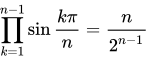
{\displaystyle \prod _{k=1}^{n-1}\sin \left({\frac {k\pi }{n}}\right)={\frac {n}{2^{n-1}}}.}
より一般的には整数 n > 0の場合 [32]
sin
(
n
x
)
=
2
n
−
1
∏
k
=
0
n
−
1
sin
(
k
n
π
+
x
)
=
2
n
−
1
∏
k
=
1
n
sin
(
k
n
π
−
x
)
.
{\displaystyle \sin(nx)=2^{n-1}\prod _{k=0}^{n-1}\sin \left({\frac {k}{n}}\pi +x\right)=2^{n-1}\prod _{k=1}^{n}\sin \left({\frac {k}{n}}\pi -x\right).}
またはコード 関数 で記述すると 、
crd
x
≡
2
sin
1
2
x
{\textstyle \operatorname {crd} x\equiv 2\sin {\tfrac {1}{2}}x}
crd
(
n
x
)
=
∏
k
=
1
n
crd
(
k
n
2
π
−
x
)
.
{\displaystyle \operatorname {crd} (nx)=\prod _{k=1}^{n}\operatorname {crd} \left({\frac {k}{n}}2\pi -x\right).}
これは多項式を 線形因数に因数分解すること から来ている( 単位根を 参照)。任意の複素数 z と整数 n > 0 に対して、
z
n
−
1
{\textstyle z^{n}-1}
z
n
−
1
=
∏
k
=
1
n
(
z
−
exp
(
k
n
2
π
i
)
)
.
{\displaystyle z^{n}-1=\prod _{k=1}^{n}\left(z-\exp {\Bigl (}{\frac {k}{n}}2\pi i{\Bigr )}\right).}
線形結合 いくつかの目的のために、同じ周期または周波数で位相シフトが異なる正弦波の線形結合は、 同じ周期または周波数で位相シフトが異なる正弦波でもあることを知っておくことが重要です。これは、 測定 または観測されたデータが以下の 同相および直交成分 基底の未知数 a および b に線形関係にあるため、および のものと比較して、 より単純な ヤコビアンが得られるため、 正弦波 データのフィッティング に役立ちます。
c
{\displaystyle c}
φ
{\displaystyle \varphi }
正弦と余弦 正弦波と余弦波の線形結合、または高調波加算は、位相シフトと振幅のスケーリングされた単一の正弦波と同等である。 [33] [34]
a
cos
x
+
b
sin
x
=
c
cos
(
x
+
φ
)
{\displaystyle a\cos x+b\sin x=c\cos(x+\varphi )}
ここで 、および は次のように定義されます。
c
{\displaystyle c}
φ
{\displaystyle \varphi }
c
=
sgn
(
a
)
a
2
+
b
2
,
φ
=
arctan
(
−
b
/
a
)
,
{\displaystyle {\begin{aligned}c&=\operatorname {sgn}(a){\sqrt {a^{2}+b^{2}}},\\\varphi &={\arctan }{\bigl (}{-b/a}{\bigr )},\end{aligned}}}
とすれば
a
≠
0.
{\displaystyle a\neq 0.}
任意の位相シフト より一般的には、任意の位相シフトに対して、
a
sin
(
x
+
θ
a
)
+
b
sin
(
x
+
θ
b
)
=
c
sin
(
x
+
φ
)
{\displaystyle a\sin(x+\theta _{a})+b\sin(x+\theta _{b})=c\sin(x+\varphi )}
ここで 、 次を満たします。
c
{\displaystyle c}
φ
{\displaystyle \varphi }
c
2
=
a
2
+
b
2
+
2
a
b
cos
(
θ
a
−
θ
b
)
,
tan
φ
=
a
sin
θ
a
+
b
sin
θ
b
a
cos
θ
a
+
b
cos
θ
b
.
{\displaystyle {\begin{aligned}c^{2}&=a^{2}+b^{2}+2ab\cos \left(\theta _{a}-\theta _{b}\right),\\\tan \varphi &={\frac {a\sin \theta _{a}+b\sin \theta _{b}}{a\cos \theta _{a}+b\cos \theta _{b}}}.\end{aligned}}}
2つ以上の正弦波 一般的なケースは次の通りである [34]
∑
i
a
i
sin
(
x
+
θ
i
)
=
a
sin
(
x
+
θ
)
,
{\displaystyle \sum _{i}a_{i}\sin(x+\theta _{i})=a\sin(x+\theta ),}
どこで
そして
a
2
=
∑
i
,
j
a
i
a
j
cos
(
θ
i
−
θ
j
)
{\displaystyle a^{2}=\sum _{i,j}a_{i}a_{j}\cos(\theta _{i}-\theta _{j})}
tan
θ
=
∑
i
a
i
sin
θ
i
∑
i
a
i
cos
θ
i
.
{\displaystyle \tan \theta ={\frac {\sum _{i}a_{i}\sin \theta _{i}}{\sum _{i}a_{i}\cos \theta _{i}}}.}
ラグランジュの三角関数の恒等式 これらの恒等式は、 ジョゼフ・ルイ・ラグランジュ にちなんで名付けられており、
以下の通り である。 [35] [36] [37]
∑
k
=
0
n
sin
k
θ
=
cos
1
2
θ
−
cos
(
(
n
+
1
2
)
θ
)
2
sin
1
2
θ
∑
k
=
0
n
cos
k
θ
=
sin
1
2
θ
+
sin
(
(
n
+
1
2
)
θ
)
2
sin
1
2
θ
{\displaystyle {\begin{aligned}\sum _{k=0}^{n}\sin k\theta &={\frac {\cos {\tfrac {1}{2}}\theta -\cos \left(\left(n+{\tfrac {1}{2}}\right)\theta \right)}{2\sin {\tfrac {1}{2}}\theta }}\\[5pt]\sum _{k=0}^{n}\cos k\theta &={\frac {\sin {\tfrac {1}{2}}\theta +\sin \left(\left(n+{\tfrac {1}{2}}\right)\theta \right)}{2\sin {\tfrac {1}{2}}\theta }}\end{aligned}}}
θ
≢
0
(
mod
2
π
)
.
{\displaystyle \theta \not \equiv 0{\pmod {2\pi }}.}
関連する関数として ディリクレ核 がある。
D
n
(
θ
)
=
1
+
2
∑
k
=
1
n
cos
k
θ
=
sin
(
(
n
+
1
2
)
θ
)
sin
1
2
θ
.
{\displaystyle D_{n}(\theta )=1+2\sum _{k=1}^{n}\cos k\theta ={\frac {\sin \left(\left(n+{\tfrac {1}{2}}\right)\theta \right)}{\sin {\tfrac {1}{2}}\theta }}.}
同様のアイデンティティは [38]
∑
k
=
1
n
cos
(
2
k
−
1
)
α
=
sin
(
2
n
α
)
2
sin
α
.
{\displaystyle \sum _{k=1}^{n}\cos(2k-1)\alpha ={\frac {\sin(2n\alpha )}{2\sin \alpha }}.}
証明は次の通りです。角度の和と差の恒等式を使って、
次の式を調べてみましょう。
sin
(
A
+
B
)
−
sin
(
A
−
B
)
=
2
cos
A
sin
B
.
{\displaystyle \sin(A+B)-\sin(A-B)=2\cos A\sin B.}
2
sin
α
∑
k
=
1
n
cos
(
2
k
−
1
)
α
=
2
sin
α
cos
α
+
2
sin
α
cos
3
α
+
2
sin
α
cos
5
α
+
…
+
2
sin
α
cos
(
2
n
−
1
)
α
{\displaystyle 2\sin \alpha \sum _{k=1}^{n}\cos(2k-1)\alpha =2\sin \alpha \cos \alpha +2\sin \alpha \cos 3\alpha +2\sin \alpha \cos 5\alpha +\ldots +2\sin \alpha \cos(2n-1)\alpha }
この式は上記の等式を使って次のように書くことができる。
2
sin
α
∑
k
=
1
n
cos
(
2
k
−
1
)
α
=
∑
k
=
1
n
(
sin
(
2
k
α
)
−
sin
(
2
(
k
−
1
)
α
)
)
=
(
sin
2
α
−
sin
0
)
+
(
sin
4
α
−
sin
2
α
)
+
(
sin
6
α
−
sin
4
α
)
+
…
+
(
sin
(
2
n
α
)
−
sin
(
2
(
n
−
1
)
α
)
)
=
sin
(
2
n
α
)
.
{\displaystyle {\begin{aligned}&2\sin \alpha \sum _{k=1}^{n}\cos(2k-1)\alpha \\&\quad =\sum _{k=1}^{n}(\sin(2k\alpha )-\sin(2(k-1)\alpha ))\\&\quad =(\sin 2\alpha -\sin 0)+(\sin 4\alpha -\sin 2\alpha )+(\sin 6\alpha -\sin 4\alpha )+\ldots +(\sin(2n\alpha )-\sin(2(n-1)\alpha ))\\&\quad =\sin(2n\alpha ).\end{aligned}}}
したがって、この式を で割ると 証明が完了します。
2
sin
α
{\displaystyle 2\sin \alpha }
が 線形分数変換 で与えられ
、同様
に
f
(
x
)
{\displaystyle f(x)}
f
(
x
)
=
(
cos
α
)
x
−
sin
α
(
sin
α
)
x
+
cos
α
,
{\displaystyle f(x)={\frac {(\cos \alpha )x-\sin \alpha }{(\sin \alpha )x+\cos \alpha }},}
g
(
x
)
=
(
cos
β
)
x
−
sin
β
(
sin
β
)
x
+
cos
β
,
{\displaystyle g(x)={\frac {(\cos \beta )x-\sin \beta }{(\sin \beta )x+\cos \beta }},}
f
(
g
(
x
)
)
=
g
(
f
(
x
)
)
=
(
cos
(
α
+
β
)
)
x
−
sin
(
α
+
β
)
(
sin
(
α
+
β
)
)
x
+
cos
(
α
+
β
)
.
{\displaystyle f{\big (}g(x){\big )}=g{\big (}f(x){\big )}={\frac {{\big (}\cos(\alpha +\beta ){\big )}x-\sin(\alpha +\beta )}{{\big (}\sin(\alpha +\beta ){\big )}x+\cos(\alpha +\beta )}}.}
もっと簡潔に言えば、もし私たち が上で述べたことをすべて 認めるならば 、
α
{\displaystyle \alpha }
f
α
{\displaystyle f_{\alpha }}
f
{\displaystyle f}
f
α
∘
f
β
=
f
α
+
β
.
{\displaystyle f_{\alpha }\circ f_{\beta }=f_{\alpha +\beta }.}
が直線の傾きである 場合、 は その直線を角度 で回転させた傾きです。
x
{\displaystyle x}
f
(
x
)
{\displaystyle f(x)}
−
α
.
{\displaystyle -\alpha .}
複素指数関数との関係 オイラーの公式によれば、任意の実数 xに対して [39]、 i は 虚数単位
で ある 。x に −xを 代入すると 次のようになる。
e
i
x
=
cos
x
+
i
sin
x
,
{\displaystyle e^{ix}=\cos x+i\sin x,}
e
−
i
x
=
cos
(
−
x
)
+
i
sin
(
−
x
)
=
cos
x
−
i
sin
x
.
{\displaystyle e^{-ix}=\cos(-x)+i\sin(-x)=\cos x-i\sin x.}
これら2つの方程式は、指数関数 を用いてコサインとサインを求めるのに使えます 。具体的には、 [40] [41]
cos
x
=
e
i
x
+
e
−
i
x
2
{\displaystyle \cos x={\frac {e^{ix}+e^{-ix}}{2}}}
sin
x
=
e
i
x
−
e
−
i
x
2
i
{\displaystyle \sin x={\frac {e^{ix}-e^{-ix}}{2i}}}
これらの公式は他の多くの三角関数の等式を証明するのに有用である。例えば、
e i ( θ + φ ) = e iθ e iφ は、
cos( θ + φ ) + i sin( θ + φ ) = (cos θ + i sin θ ) (cos φ + i sin φ ) = (cos θ cos φ − sin θ sin φ ) + i (cos θ sin φ +sin θ cos φ ) 。
左辺の実部が右辺の実部に等しいことは、コサインの角度の加算公式です。虚部が等しいことは、サインの角度の加算公式になります。
次の表は、三角関数とその逆関数を指数関数と複素対数 で表したものです 。
複素双曲線関数との関係 三角関数は複素 引数を持つ 双曲関数 から演繹される 。その関係式を以下に示す [43] [44] 。
sin
x
=
−
i
sinh
(
i
x
)
cos
x
=
cosh
(
i
x
)
tan
x
=
−
i
tanh
(
i
x
)
cot
x
=
i
coth
(
i
x
)
sec
x
=
sech
(
i
x
)
csc
x
=
i
csch
(
i
x
)
{\displaystyle {\begin{aligned}\sin x&=-i\sinh(ix)\\\cos x&=\cosh(ix)\\\tan x&=-i\tanh(ix)\\\cot x&=i\coth(ix)\\\sec x&=\operatorname {sech} (ix)\\\csc x&=i\operatorname {csch} (ix)\\\end{aligned}}}
シリーズ拡大 三角関数を定義するためにべき級数 展開を使用すると 、次の恒等式が得られます。 [45]
sin
x
=
x
−
x
3
3
!
+
x
5
5
!
−
x
7
7
!
+
⋯
=
∑
n
=
0
∞
(
−
1
)
n
x
2
n
+
1
(
2
n
+
1
)
!
,
{\displaystyle \sin x=x-{\frac {x^{3}}{3!}}+{\frac {x^{5}}{5!}}-{\frac {x^{7}}{7!}}+\cdots =\sum _{n=0}^{\infty }{\frac {(-1)^{n}x^{2n+1}}{(2n+1)!}},}
cos
x
=
1
−
x
2
2
!
+
x
4
4
!
−
x
6
6
!
+
⋯
=
∑
n
=
0
∞
(
−
1
)
n
x
2
n
(
2
n
)
!
.
{\displaystyle \cos x=1-{\frac {x^{2}}{2!}}+{\frac {x^{4}}{4!}}-{\frac {x^{6}}{6!}}+\cdots =\sum _{n=0}^{\infty }{\frac {(-1)^{n}x^{2n}}{(2n)!}}.}
特殊関数 への応用では、 三角関数の 次の 無限積公式が有用である: [46] [47]
sin
x
=
x
∏
n
=
1
∞
(
1
−
x
2
π
2
n
2
)
,
cos
x
=
∏
n
=
1
∞
(
1
−
x
2
π
2
(
n
−
1
2
)
)
2
)
,
sinh
x
=
x
∏
n
=
1
∞
(
1
+
x
2
π
2
n
2
)
,
cosh
x
=
∏
n
=
1
∞
(
1
+
x
2
π
2
(
n
−
1
2
)
)
2
)
.
{\displaystyle {\begin{aligned}\sin x&=x\prod _{n=1}^{\infty }\left(1-{\frac {x^{2}}{\pi ^{2}n^{2}}}\right),&\cos x&=\prod _{n=1}^{\infty }\left(1-{\frac {x^{2}}{\pi ^{2}\left(n-{\frac {1}{2}}\right)\!{\vphantom {)}}^{2}}}\right),\\[10mu]\sinh x&=x\prod _{n=1}^{\infty }\left(1+{\frac {x^{2}}{\pi ^{2}n^{2}}}\right),&\cosh x&=\prod _{n=1}^{\infty }\left(1+{\frac {x^{2}}{\pi ^{2}\left(n-{\frac {1}{2}}\right)\!{\vphantom {)}}^{2}}}\right).\end{aligned}}}
逆三角関数 次の等式は三角関数と逆三角関数を合成した結果を与える。 [48]
sin
(
arcsin
x
)
=
x
cos
(
arcsin
x
)
=
1
−
x
2
tan
(
arcsin
x
)
=
x
1
−
x
2
sin
(
arccos
x
)
=
1
−
x
2
cos
(
arccos
x
)
=
x
tan
(
arccos
x
)
=
1
−
x
2
x
sin
(
arctan
x
)
=
x
1
+
x
2
cos
(
arctan
x
)
=
1
1
+
x
2
tan
(
arctan
x
)
=
x
sin
(
arccsc
x
)
=
1
x
cos
(
arccsc
x
)
=
x
2
−
1
x
tan
(
arccsc
x
)
=
1
x
2
−
1
sin
(
arcsec
x
)
=
x
2
−
1
x
cos
(
arcsec
x
)
=
1
x
tan
(
arcsec
x
)
=
x
2
−
1
sin
(
arccot
x
)
=
1
1
+
x
2
cos
(
arccot
x
)
=
x
1
+
x
2
tan
(
arccot
x
)
=
1
x
{\displaystyle {\begin{aligned}\sin(\arcsin x)&=x&\cos(\arcsin x)&={\sqrt {1-x^{2}}}&\tan(\arcsin x)&={\frac {x}{\sqrt {1-x^{2}}}}\\\sin(\arccos x)&={\sqrt {1-x^{2}}}&\cos(\arccos x)&=x&\tan(\arccos x)&={\frac {\sqrt {1-x^{2}}}{x}}\\\sin(\arctan x)&={\frac {x}{\sqrt {1+x^{2}}}}&\cos(\arctan x)&={\frac {1}{\sqrt {1+x^{2}}}}&\tan(\arctan x)&=x\\\sin(\operatorname {arccsc} x)&={\frac {1}{x}}&\cos(\operatorname {arccsc} x)&={\frac {\sqrt {x^{2}-1}}{x}}&\tan(\operatorname {arccsc} x)&={\frac {1}{\sqrt {x^{2}-1}}}\\\sin(\operatorname {arcsec} x)&={\frac {\sqrt {x^{2}-1}}{x}}&\cos(\operatorname {arcsec} x)&={\frac {1}{x}}&\tan(\operatorname {arcsec} x)&={\sqrt {x^{2}-1}}\\\sin(\operatorname {arccot} x)&={\frac {1}{\sqrt {1+x^{2}}}}&\cos(\operatorname {arccot} x)&={\frac {x}{\sqrt {1+x^{2}}}}&\tan(\operatorname {arccot} x)&={\frac {1}{x}}\\\end{aligned}}}
上記の各式の両辺の 逆数を 取ると、 の式が得られます
。 上記の式の右辺は常に反転されます。 たとえば、 の式は次のように なります。
一方、 との
式は次のようになります 。
csc
=
1
sin
,
sec
=
1
cos
,
and
cot
=
1
tan
.
{\displaystyle \csc ={\frac {1}{\sin }},\;\sec ={\frac {1}{\cos }},{\text{ and }}\cot ={\frac {1}{\tan }}.}
cot
(
arcsin
x
)
{\displaystyle \cot(\arcsin x)}
cot
(
arcsin
x
)
=
1
tan
(
arcsin
x
)
=
1
x
1
−
x
2
=
1
−
x
2
x
{\displaystyle \cot(\arcsin x)={\frac {1}{\tan(\arcsin x)}}={\frac {1}{\frac {x}{\sqrt {1-x^{2}}}}}={\frac {\sqrt {1-x^{2}}}{x}}}
csc
(
arccos
x
)
{\displaystyle \csc(\arccos x)}
sec
(
arccos
x
)
{\displaystyle \sec(\arccos x)}
csc
(
arccos
x
)
=
1
sin
(
arccos
x
)
=
1
1
−
x
2
and
sec
(
arccos
x
)
=
1
cos
(
arccos
x
)
=
1
x
.
{\displaystyle \csc(\arccos x)={\frac {1}{\sin(\arccos x)}}={\frac {1}{\sqrt {1-x^{2}}}}\qquad {\text{ and }}\quad \sec(\arccos x)={\frac {1}{\cos(\arccos x)}}={\frac {1}{x}}.}
反射恒等式によって次の恒等式が暗示されます。これらは、 関連する関数のドメイン内にあるときは常に成立します。
x
,
r
,
s
,
−
x
,
−
r
,
and
−
s
{\displaystyle x,r,s,-x,-r,{\text{ and }}-s}
π
2
=
arcsin
(
x
)
+
arccos
(
x
)
=
arctan
(
r
)
+
arccot
(
r
)
=
arcsec
(
s
)
+
arccsc
(
s
)
π
=
arccos
(
x
)
+
arccos
(
−
x
)
=
arccot
(
r
)
+
arccot
(
−
r
)
=
arcsec
(
s
)
+
arcsec
(
−
s
)
0
=
arcsin
(
x
)
+
arcsin
(
−
x
)
=
arctan
(
r
)
+
arctan
(
−
r
)
=
arccsc
(
s
)
+
arccsc
(
−
s
)
{\displaystyle {\begin{alignedat}{9}{\frac {\pi }{2}}~&=~\arcsin(x)&&+\arccos(x)~&&=~\arctan(r)&&+\operatorname {arccot}(r)~&&=~\operatorname {arcsec}(s)&&+\operatorname {arccsc}(s)\\[0.4ex]\pi ~&=~\arccos(x)&&+\arccos(-x)~&&=~\operatorname {arccot}(r)&&+\operatorname {arccot}(-r)~&&=~\operatorname {arcsec}(s)&&+\operatorname {arcsec}(-s)\\[0.4ex]0~&=~\arcsin(x)&&+\arcsin(-x)~&&=~\arctan(r)&&+\arctan(-r)~&&=~\operatorname {arccsc}(s)&&+\operatorname {arccsc}(-s)\\[1.0ex]\end{alignedat}}}
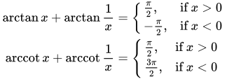
また、 [49]
arctan
x
+
arctan
1
x
=
{
π
2
,
if
x
>
0
−
π
2
,
if
x
<
0
arccot
x
+
arccot
1
x
=
{
π
2
,
if
x
>
0
3
π
2
,
if
x
<
0
{\displaystyle {\begin{aligned}\arctan x+\arctan {\dfrac {1}{x}}&={\begin{cases}{\frac {\pi }{2}},&{\text{if }}x>0\\-{\frac {\pi }{2}},&{\text{if }}x<0\end{cases}}\\\operatorname {arccot} x+\operatorname {arccot} {\dfrac {1}{x}}&={\begin{cases}{\frac {\pi }{2}},&{\text{if }}x>0\\{\frac {3\pi }{2}},&{\text{if }}x<0\end{cases}}\\\end{aligned}}}
arccos
1
x
=
arcsec
x
and
arcsec
1
x
=
arccos
x
{\displaystyle \arccos {\frac {1}{x}}=\operatorname {arcsec} x\qquad {\text{ and }}\qquad \operatorname {arcsec} {\frac {1}{x}}=\arccos x}
arcsin
1
x
=
arccsc
x
and
arccsc
1
x
=
arcsin
x
{\displaystyle \arcsin {\frac {1}{x}}=\operatorname {arccsc} x\qquad {\text{ and }}\qquad \operatorname {arccsc} {\frac {1}{x}}=\arcsin x}
逆正接 関数 は級数的に展開できる: [50]
arctan
(
n
x
)
=
∑
m
=
1
n
arctan
x
1
+
(
m
−
1
)
m
x
2
{\displaystyle \arctan(nx)=\sum _{m=1}^{n}\arctan {\frac {x}{1+(m-1)mx^{2}}}}
変数のないアイデンティティ 逆正接 関数 に関しては [49]
arctan
1
2
=
arctan
1
3
+
arctan
1
7
.
{\displaystyle \arctan {\frac {1}{2}}=\arctan {\frac {1}{3}}+\arctan {\frac {1}{7}}.}
モリーの法則 として知られる奇妙な同一性 、
cos
20
∘
⋅
cos
40
∘
⋅
cos
80
∘
=
1
8
,
{\displaystyle \cos 20^{\circ }\cdot \cos 40^{\circ }\cdot \cos 80^{\circ }={\frac {1}{8}},}
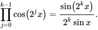
は、1 つの変数を含む恒等式の特殊なケースです。
∏
j
=
0
k
−
1
cos
(
2
j
x
)
=
sin
(
2
k
x
)
2
k
sin
x
.
{\displaystyle \prod _{j=0}^{k-1}\cos \left(2^{j}x\right)={\frac {\sin \left(2^{k}x\right)}{2^{k}\sin x}}.}
同様に、
は との恒等式の特殊なケースです 。
sin
20
∘
⋅
sin
40
∘
⋅
sin
80
∘
=
3
8
{\displaystyle \sin 20^{\circ }\cdot \sin 40^{\circ }\cdot \sin 80^{\circ }={\frac {\sqrt {3}}{8}}}
x
=
20
∘
{\displaystyle x=20^{\circ }}
sin
x
⋅
sin
(
60
∘
−
x
)
⋅
sin
(
60
∘
+
x
)
=
sin
3
x
4
.
{\displaystyle \sin x\cdot \sin \left(60^{\circ }-x\right)\cdot \sin \left(60^{\circ }+x\right)={\frac {\sin 3x}{4}}.}
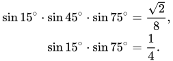
この場合 、
x
=
15
∘
{\displaystyle x=15^{\circ }}
sin
15
∘
⋅
sin
45
∘
⋅
sin
75
∘
=
2
8
,
sin
15
∘
⋅
sin
75
∘
=
1
4
.
{\displaystyle {\begin{aligned}\sin 15^{\circ }\cdot \sin 45^{\circ }\cdot \sin 75^{\circ }&={\frac {\sqrt {2}}{8}},\\\sin 15^{\circ }\cdot \sin 75^{\circ }&={\frac {1}{4}}.\end{aligned}}}
この場合 、
x
=
10
∘
{\displaystyle x=10^{\circ }}
sin
10
∘
⋅
sin
50
∘
⋅
sin
70
∘
=
1
8
.
{\displaystyle \sin 10^{\circ }\cdot \sin 50^{\circ }\cdot \sin 70^{\circ }={\frac {1}{8}}.}
同じコサイン恒等式は
cos
x
⋅
cos
(
60
∘
−
x
)
⋅
cos
(
60
∘
+
x
)
=
cos
3
x
4
.
{\displaystyle \cos x\cdot \cos \left(60^{\circ }-x\right)\cdot \cos \left(60^{\circ }+x\right)={\frac {\cos 3x}{4}}.}
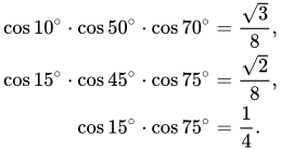
同様に、
cos
10
∘
⋅
cos
50
∘
⋅
cos
70
∘
=
3
8
,
cos
15
∘
⋅
cos
45
∘
⋅
cos
75
∘
=
2
8
,
cos
15
∘
⋅
cos
75
∘
=
1
4
.
{\displaystyle {\begin{aligned}\cos 10^{\circ }\cdot \cos 50^{\circ }\cdot \cos 70^{\circ }&={\frac {\sqrt {3}}{8}},\\\cos 15^{\circ }\cdot \cos 45^{\circ }\cdot \cos 75^{\circ }&={\frac {\sqrt {2}}{8}},\\\cos 15^{\circ }\cdot \cos 75^{\circ }&={\frac {1}{4}}.\end{aligned}}}
同様に、
tan
50
∘
⋅
tan
60
∘
⋅
tan
70
∘
=
tan
80
∘
,
tan
40
∘
⋅
tan
30
∘
⋅
tan
20
∘
=
tan
10
∘
.
{\displaystyle {\begin{aligned}\tan 50^{\circ }\cdot \tan 60^{\circ }\cdot \tan 70^{\circ }&=\tan 80^{\circ },\\\tan 40^{\circ }\cdot \tan 30^{\circ }\cdot \tan 20^{\circ }&=\tan 10^{\circ }.\end{aligned}}}
以下は、変数を含む恒等式に簡単に一般化できるものではないかもしれません (ただし、以下の説明を参照してください)。
cos
24
∘
+
cos
48
∘
+
cos
96
∘
+
cos
168
∘
=
1
2
.
{\displaystyle \cos 24^{\circ }+\cos 48^{\circ }+\cos 96^{\circ }+\cos 168^{\circ }={\frac {1}{2}}.}
分母が 21 であるこの等式を考慮すると、度測定はラジアン測定よりも適切ではなくなります。
cos
2
π
21
+
cos
(
2
⋅
2
π
21
)
+
cos
(
4
⋅
2
π
21
)
+
cos
(
5
⋅
2
π
21
)
+
cos
(
8
⋅
2
π
21
)
+
cos
(
10
⋅
2
π
21
)
=
1
2
.
{\displaystyle \cos {\frac {2\pi }{21}}+\cos \left(2\cdot {\frac {2\pi }{21}}\right)+\cos \left(4\cdot {\frac {2\pi }{21}}\right)+\cos \left(5\cdot {\frac {2\pi }{21}}\right)+\cos \left(8\cdot {\frac {2\pi }{21}}\right)+\cos \left(10\cdot {\frac {2\pi }{21}}\right)={\frac {1}{2}}.}
1、2、4、5、8、10という因数からパターンが明らかになるかもしれません。これらは、 より小さい整数です。 21 / 2 は 21 と互いに素 である(または 共通の 素因数 を持たない)。最後のいくつかの例は、既約 円分多項式 に関する基本的事実の帰結です。つまり、余弦はそれらの多項式の零点の実数部であり、零点の合計は(上記の最後のケースでは)21 で評価された メビウス関数 であり、上記には零点の半分だけが存在しています。この最後の例の前の 2 つの恒等式は、21 をそれぞれ 10 と 15 に置き換えて同じように生じます。
その他のコサイン恒等式には以下が含まれる: [51]
奇数すべてに対して同様であり、したがって
2
cos
π
3
=
1
,
2
cos
π
5
×
2
cos
2
π
5
=
1
,
2
cos
π
7
×
2
cos
2
π
7
×
2
cos
3
π
7
=
1
,
{\displaystyle {\begin{aligned}2\cos {\frac {\pi }{3}}&=1,\\2\cos {\frac {\pi }{5}}\times 2\cos {\frac {2\pi }{5}}&=1,\\2\cos {\frac {\pi }{7}}\times 2\cos {\frac {2\pi }{7}}\times 2\cos {\frac {3\pi }{7}}&=1,\end{aligned}}}
cos
π
3
+
cos
π
5
×
cos
2
π
5
+
cos
π
7
×
cos
2
π
7
×
cos
3
π
7
+
⋯
=
1.
{\displaystyle \cos {\frac {\pi }{3}}+\cos {\frac {\pi }{5}}\times \cos {\frac {2\pi }{5}}+\cos {\frac {\pi }{7}}\times \cos {\frac {2\pi }{7}}\times \cos {\frac {3\pi }{7}}+\dots =1.}
これらの奇妙なアイデンティティの多くは、次のようなより一般的な事実から生じています。 [52
]
∏
k
=
1
n
−
1
sin
k
π
n
=
n
2
n
−
1
{\displaystyle \prod _{k=1}^{n-1}\sin {\frac {k\pi }{n}}={\frac {n}{2^{n-1}}}}
∏
k
=
1
n
−
1
cos
k
π
n
=
sin
π
n
2
2
n
−
1
.
{\displaystyle \prod _{k=1}^{n-1}\cos {\frac {k\pi }{n}}={\frac {\sin {\frac {\pi n}{2}}}{2^{n-1}}}.}
これらを組み合わせると
∏
k
=
1
n
−
1
tan
k
π
n
=
n
sin
π
n
2
{\displaystyle \prod _{k=1}^{n-1}\tan {\frac {k\pi }{n}}={\frac {n}{\sin {\frac {\pi n}{2}}}}}
n が奇数( )の 場合 には対称性を利用して
n
=
2
m
+
1
{\displaystyle n=2m+1}
∏
k
=
1
m
tan
k
π
2
m
+
1
=
2
m
+
1
{\displaystyle \prod _{k=1}^{m}\tan {\frac {k\pi }{2m+1}}={\sqrt {2m+1}}}
バターワース ローパス フィルタ の伝達関数は 、多項式と極で表すことができます。周波数をカットオフ周波数として設定すると、次の恒等式が証明されます。
∏
k
=
1
n
sin
(
2
k
−
1
)
π
4
n
=
∏
k
=
1
n
cos
(
2
k
−
1
)
π
4
n
=
2
2
n
{\displaystyle \prod _{k=1}^{n}\sin {\frac {\left(2k-1\right)\pi }{4n}}=\prod _{k=1}^{n}\cos {\frac {\left(2k-1\right)\pi }{4n}}={\frac {\sqrt {2}}{2^{n}}}}
コンピューティング π π を 大きな桁数 まで効率的に 計算する 方法は、 マチン による次の変数なしの恒等式に基づいています。これは マチンのような式 として知られています 。
または、 レオンハルト・オイラー
の恒等式を使用するか 、
ピタゴラスの三つ組
を使用するかのいずれかです 。
π
4
=
4
arctan
1
5
−
arctan
1
239
{\displaystyle {\frac {\pi }{4}}=4\arctan {\frac {1}{5}}-\arctan {\frac {1}{239}}}
π
4
=
5
arctan
1
7
+
2
arctan
3
79
{\displaystyle {\frac {\pi }{4}}=5\arctan {\frac {1}{7}}+2\arctan {\frac {3}{79}}}
π
=
arccos
4
5
+
arccos
5
13
+
arccos
16
65
=
arcsin
3
5
+
arcsin
12
13
+
arcsin
63
65
.
{\displaystyle \pi =\arccos {\frac {4}{5}}+\arccos {\frac {5}{13}}+\arccos {\frac {16}{65}}=\arcsin {\frac {3}{5}}+\arcsin {\frac {12}{13}}+\arcsin {\frac {63}{65}}.}
その他には以下のものがある: [53] [49]
π
4
=
arctan
1
2
+
arctan
1
3
,
{\displaystyle {\frac {\pi }{4}}=\arctan {\frac {1}{2}}+\arctan {\frac {1}{3}},}
π
=
arctan
1
+
arctan
2
+
arctan
3
,
{\displaystyle \pi =\arctan 1+\arctan 2+\arctan 3,}
π
4
=
2
arctan
1
3
+
arctan
1
7
.
{\displaystyle {\frac {\pi }{4}}=2\arctan {\frac {1}{3}}+\arctan {\frac {1}{7}}.}
一般に、 θ n = Σ となる 数 t 1 , ..., t n −1 ∈ (−1, 1)に対して、 n −1 k =1 arctan t k ∈ ( π /4, 3 π /4) 、 t n = tan( π /2 − θ n ) = cot θ n とします。この最後の式は、 t 1 、 ...、 t n −1 の正接を持つ角度の合計のコタンジェントの公式を使用して直接計算でき、その値は (-1, 1) の範囲になります 。特に、 t 1 、 ...、 t n −1の値が有理数である場合、計算された t n は 有理数になります 。これらの値を使用すると、
π
2
=
∑
k
=
1
n
arctan
(
t
k
)
π
=
∑
k
=
1
n
sgn
(
t
k
)
arccos
(
1
−
t
k
2
1
+
t
k
2
)
π
=
∑
k
=
1
n
arcsin
(
2
t
k
1
+
t
k
2
)
π
=
∑
k
=
1
n
arctan
(
2
t
k
1
−
t
k
2
)
,
{\displaystyle {\begin{aligned}{\frac {\pi }{2}}&=\sum _{k=1}^{n}\arctan(t_{k})\\\pi &=\sum _{k=1}^{n}\operatorname {sgn}(t_{k})\arccos \left({\frac {1-t_{k}^{2}}{1+t_{k}^{2}}}\right)\\\pi &=\sum _{k=1}^{n}\arcsin \left({\frac {2t_{k}}{1+t_{k}^{2}}}\right)\\\pi &=\sum _{k=1}^{n}\arctan \left({\frac {2t_{k}}{1-t_{k}^{2}}}\right)\,,\end{aligned}}}
ここで、最初の式を除くすべての式では、正接半角の公式を使用しています。最初の 2 つの式は、 t k 値の 1 つ以上が(−1, 1) の範囲外であっても機能します 。 t = p / q が有理数の場合、上記の式の (2 t 、 1 − t 2 、 1 + t 2 ) 値は、ピタゴラスの三つ組 (2 pq 、 q 2 − p 2 、 q 2 + p 2 ) に比例することに注意してください。
たとえば、 n = 3 項の場合、
任意の a 、 b 、 c 、 d > 0 です。
π
2
=
arctan
(
a
b
)
+
arctan
(
c
d
)
+
arctan
(
b
d
−
a
c
a
d
+
b
c
)
{\displaystyle {\frac {\pi }{2}}=\arctan \left({\frac {a}{b}}\right)+\arctan \left({\frac {c}{d}}\right)+\arctan \left({\frac {bd-ac}{ad+bc}}\right)}
ユークリッドの同一性 ユークリッドは『 原論 』第 13 巻命題 10 で、 円に内接する正五角形の辺にある正方形の面積は、同じ円に内接する正六角形と正十角形の辺にある正方形の面積の合計に等しいことを示しました。現代の三角法の言葉で言えば、次のようになります。
sin
2
18
∘
+
sin
2
30
∘
=
sin
2
36
∘
.
{\displaystyle \sin ^{2}18^{\circ }+\sin ^{2}30^{\circ }=\sin ^{2}36^{\circ }.}
プトレマイオスは この命題を使って、 『アルマゲスト』 第 1 巻第 11 章の 弦の表 のいくつかの角度を計算しました。
三角関数の合成 これらの恒等式は三角関数の三角関数に関係している: [54]
cos
(
t
sin
x
)
=
J
0
(
t
)
+
2
∑
k
=
1
∞
J
2
k
(
t
)
cos
(
2
k
x
)
{\displaystyle \cos(t\sin x)=J_{0}(t)+2\sum _{k=1}^{\infty }J_{2k}(t)\cos(2kx)}
sin
(
t
sin
x
)
=
2
∑
k
=
0
∞
J
2
k
+
1
(
t
)
sin
(
(
2
k
+
1
)
x
)
{\displaystyle \sin(t\sin x)=2\sum _{k=0}^{\infty }J_{2k+1}(t)\sin {\big (}(2k+1)x{\big )}}
cos
(
t
cos
x
)
=
J
0
(
t
)
+
2
∑
k
=
1
∞
(
−
1
)
k
J
2
k
(
t
)
cos
(
2
k
x
)
{\displaystyle \cos(t\cos x)=J_{0}(t)+2\sum _{k=1}^{\infty }(-1)^{k}J_{2k}(t)\cos(2kx)}
sin
(
t
cos
x
)
=
2
∑
k
=
0
∞
(
−
1
)
k
J
2
k
+
1
(
t
)
cos
(
(
2
k
+
1
)
x
)
{\displaystyle \sin(t\cos x)=2\sum _{k=0}^{\infty }(-1)^{k}J_{2k+1}(t)\cos {\big (}(2k+1)x{\big )}}
ここで、 J i は ベッセル関数 です 。
このケースのさらなる「条件付き」アイデンティティ α + β + γ = 180° 条件付き三角関数恒等式 は 、三角関数の引数に指定された条件が満たされる場合に成立する三角関数恒等式である。 [55] 次の公式は任意の平面三角形に適用され、 公式に現れる関数が明確に定義されている限り、から導かれる(後者は正接と余接が現れる公式にのみ適用される)。
α
+
β
+
γ
=
180
∘
,
{\displaystyle \alpha +\beta +\gamma =180^{\circ },}
tan
α
+
tan
β
+
tan
γ
=
tan
α
tan
β
tan
γ
1
=
cot
β
cot
γ
+
cot
γ
cot
α
+
cot
α
cot
β
cot
(
α
2
)
+
cot
(
β
2
)
+
cot
(
γ
2
)
=
cot
(
α
2
)
cot
(
β
2
)
cot
(
γ
2
)
1
=
tan
(
β
2
)
tan
(
γ
2
)
+
tan
(
γ
2
)
tan
(
α
2
)
+
tan
(
α
2
)
tan
(
β
2
)
sin
α
+
sin
β
+
sin
γ
=
4
cos
(
α
2
)
cos
(
β
2
)
cos
(
γ
2
)
−
sin
α
+
sin
β
+
sin
γ
=
4
cos
(
α
2
)
sin
(
β
2
)
sin
(
γ
2
)
cos
α
+
cos
β
+
cos
γ
=
4
sin
(
α
2
)
sin
(
β
2
)
sin
(
γ
2
)
+
1
−
cos
α
+
cos
β
+
cos
γ
=
4
sin
(
α
2
)
cos
(
β
2
)
cos
(
γ
2
)
−
1
sin
(
2
α
)
+
sin
(
2
β
)
+
sin
(
2
γ
)
=
4
sin
α
sin
β
sin
γ
−
sin
(
2
α
)
+
sin
(
2
β
)
+
sin
(
2
γ
)
=
4
sin
α
cos
β
cos
γ
cos
(
2
α
)
+
cos
(
2
β
)
+
cos
(
2
γ
)
=
−
4
cos
α
cos
β
cos
γ
−
1
−
cos
(
2
α
)
+
cos
(
2
β
)
+
cos
(
2
γ
)
=
−
4
cos
α
sin
β
sin
γ
+
1
sin
2
α
+
sin
2
β
+
sin
2
γ
=
2
cos
α
cos
β
cos
γ
+
2
−
sin
2
α
+
sin
2
β
+
sin
2
γ
=
2
cos
α
sin
β
sin
γ
cos
2
α
+
cos
2
β
+
cos
2
γ
=
−
2
cos
α
cos
β
cos
γ
+
1
−
cos
2
α
+
cos
2
β
+
cos
2
γ
=
−
2
cos
α
sin
β
sin
γ
+
1
sin
2
(
2
α
)
+
sin
2
(
2
β
)
+
sin
2
(
2
γ
)
=
−
2
cos
(
2
α
)
cos
(
2
β
)
cos
(
2
γ
)
+
2
cos
2
(
2
α
)
+
cos
2
(
2
β
)
+
cos
2
(
2
γ
)
=
2
cos
(
2
α
)
cos
(
2
β
)
cos
(
2
γ
)
+
1
1
=
sin
2
(
α
2
)
+
sin
2
(
β
2
)
+
sin
2
(
γ
2
)
+
2
sin
(
α
2
)
sin
(
β
2
)
sin
(
γ
2
)
{\displaystyle {\begin{aligned}\tan \alpha +\tan \beta +\tan \gamma &=\tan \alpha \tan \beta \tan \gamma \\1&=\cot \beta \cot \gamma +\cot \gamma \cot \alpha +\cot \alpha \cot \beta \\\cot \left({\frac {\alpha }{2}}\right)+\cot \left({\frac {\beta }{2}}\right)+\cot \left({\frac {\gamma }{2}}\right)&=\cot \left({\frac {\alpha }{2}}\right)\cot \left({\frac {\beta }{2}}\right)\cot \left({\frac {\gamma }{2}}\right)\\1&=\tan \left({\frac {\beta }{2}}\right)\tan \left({\frac {\gamma }{2}}\right)+\tan \left({\frac {\gamma }{2}}\right)\tan \left({\frac {\alpha }{2}}\right)+\tan \left({\frac {\alpha }{2}}\right)\tan \left({\frac {\beta }{2}}\right)\\\sin \alpha +\sin \beta +\sin \gamma &=4\cos \left({\frac {\alpha }{2}}\right)\cos \left({\frac {\beta }{2}}\right)\cos \left({\frac {\gamma }{2}}\right)\\-\sin \alpha +\sin \beta +\sin \gamma &=4\cos \left({\frac {\alpha }{2}}\right)\sin \left({\frac {\beta }{2}}\right)\sin \left({\frac {\gamma }{2}}\right)\\\cos \alpha +\cos \beta +\cos \gamma &=4\sin \left({\frac {\alpha }{2}}\right)\sin \left({\frac {\beta }{2}}\right)\sin \left({\frac {\gamma }{2}}\right)+1\\-\cos \alpha +\cos \beta +\cos \gamma &=4\sin \left({\frac {\alpha }{2}}\right)\cos \left({\frac {\beta }{2}}\right)\cos \left({\frac {\gamma }{2}}\right)-1\\\sin(2\alpha )+\sin(2\beta )+\sin(2\gamma )&=4\sin \alpha \sin \beta \sin \gamma \\-\sin(2\alpha )+\sin(2\beta )+\sin(2\gamma )&=4\sin \alpha \cos \beta \cos \gamma \\\cos(2\alpha )+\cos(2\beta )+\cos(2\gamma )&=-4\cos \alpha \cos \beta \cos \gamma -1\\-\cos(2\alpha )+\cos(2\beta )+\cos(2\gamma )&=-4\cos \alpha \sin \beta \sin \gamma +1\\\sin ^{2}\alpha +\sin ^{2}\beta +\sin ^{2}\gamma &=2\cos \alpha \cos \beta \cos \gamma +2\\-\sin ^{2}\alpha +\sin ^{2}\beta +\sin ^{2}\gamma &=2\cos \alpha \sin \beta \sin \gamma \\\cos ^{2}\alpha +\cos ^{2}\beta +\cos ^{2}\gamma &=-2\cos \alpha \cos \beta \cos \gamma +1\\-\cos ^{2}\alpha +\cos ^{2}\beta +\cos ^{2}\gamma &=-2\cos \alpha \sin \beta \sin \gamma +1\\\sin ^{2}(2\alpha )+\sin ^{2}(2\beta )+\sin ^{2}(2\gamma )&=-2\cos(2\alpha )\cos(2\beta )\cos(2\gamma )+2\\\cos ^{2}(2\alpha )+\cos ^{2}(2\beta )+\cos ^{2}(2\gamma )&=2\cos(2\alpha )\,\cos(2\beta )\,\cos(2\gamma )+1\\1&=\sin ^{2}\left({\frac {\alpha }{2}}\right)+\sin ^{2}\left({\frac {\beta }{2}}\right)+\sin ^{2}\left({\frac {\gamma }{2}}\right)+2\sin \left({\frac {\alpha }{2}}\right)\,\sin \left({\frac {\beta }{2}}\right)\,\sin \left({\frac {\gamma }{2}}\right)\end{aligned}}}
歴史的な速記法 正弦 、 カバーサイン 、 半正弦 、 および 正割は 航海に使用されていました。たとえば、 半正弦の公式は 球面上の 2 点間の距離を計算するために使用されていました。現在ではほとんど使用されていません。
その他
ディリクレ核 ディリクレ 核 D n ( x ) は、次の恒等式の両辺に現れる関数である。
1
+
2
cos
x
+
2
cos
(
2
x
)
+
2
cos
(
3
x
)
+
⋯
+
2
cos
(
n
x
)
=
sin
(
(
n
+
1
2
)
x
)
sin
(
1
2
x
)
.
{\displaystyle 1+2\cos x+2\cos(2x)+2\cos(3x)+\cdots +2\cos(nx)={\frac {\sin \left(\left(n+{\frac {1}{2}}\right)x\right)}{\sin \left({\frac {1}{2}}x\right)}}.}
周期の任意の 積分可能関数 とディリクレ核 の 畳み込み は 、関数の次のフーリエ近似と一致します。任意の 測度 または 一般化関数 についても同じことが言えます。
2
π
{\displaystyle 2\pi }
n
{\displaystyle n}
接線半角置換 とする と [56] 、 cis x と略されることも
ある 。
t
=
tan
x
2
,
{\displaystyle t=\tan {\frac {x}{2}},}
sin
x
=
2
t
1
+
t
2
;
cos
x
=
1
−
t
2
1
+
t
2
;
e
i
x
=
1
+
i
t
1
−
i
t
;
d
x
=
2
d
t
1
+
t
2
,
{\displaystyle \sin x={\frac {2t}{1+t^{2}}};\qquad \cos x={\frac {1-t^{2}}{1+t^{2}}};\qquad e^{ix}={\frac {1+it}{1-it}};\qquad dx={\frac {2\,dt}{1+t^{2}}},}
e
i
x
=
cos
x
+
i
sin
x
,
{\displaystyle e^{ix}=\cos x+i\sin x,}
tan を に 置き換えると、
t
{\displaystyle t}
x / 2 は微積分 で使用されているため 、 は に置き換えられ
sin
x
{\displaystyle \sin x}
2 トン / 1 + 2 です は に 置き換えられます
cos
x
{\displaystyle \cos x}
1 − t 2 / 1 + 2 です そして微分 d x は に置き換えられます 2 日 / 1 + 2 です . これにより、および の有理関数を の 有理関数に 変換して、それらの不定積分 を求めることができます 。
sin
x
{\displaystyle \sin x}
cos
x
{\displaystyle \cos x}
t
{\displaystyle t}
ヴィエトの無限積
cos
θ
2
⋅
cos
θ
4
⋅
cos
θ
8
⋯
=
∏
n
=
1
∞
cos
θ
2
n
=
sin
θ
θ
=
sinc
θ
.
{\displaystyle \cos {\frac {\theta }{2}}\cdot \cos {\frac {\theta }{4}}\cdot \cos {\frac {\theta }{8}}\cdots =\prod _{n=1}^{\infty }\cos {\frac {\theta }{2^{n}}}={\frac {\sin \theta }{\theta }}=\operatorname {sinc} \theta .}
参照
参考文献
^ アブラモウィッツ、ミルトン 、 ステグン、アイリーン・アン 編 (1983) [1964 年 6 月]。「第 4 章、式 4.3.45」。 数式、グラフ、および数学表付き数学関数ハンドブック 。応用数学シリーズ。第 55 巻 (訂正を含む第 10 回目の初版 (1972 年 12 月) の追加訂正を含む第 9 回目の再版、初版)。ワシントン DC、ニューヨーク: 米国商務省、国立標準局、ドーバー出版。p. 73。ISBN 978-0-486-61272-0 LCCN 64-60036。MR 0167642。LCCN 65-12253 。 ^ セルビー 1970、188 ページ ^ アブラモヴィッツとステガン、p. 72、4.3.13–15 ^ アブラモヴィッツとステガン、p. 72、4.3.7–9 ^ アブラモヴィッツとステガン、p. 72、4.3.16 ^ abcd Weisstein、Eric W. 「三角関数の加算公式」 。MathWorld 。 ^ アブラモヴィッツとステガン、p. 72、4.3.17 ^ アブラモヴィッツとステガン、p. 72、4.3.18 ^ ab 「角度の和と差の恒等式」 www.milefoot.com . 2019年10月12日 閲覧 。 ^ アブラモヴィッツとステガン、p. 72、4.3.19 ^ アブラモヴィッツとステガン、p. 80、4.4.32 ^ アブラモヴィッツとステガン、p. 80、4.4.33 ^ アブラモヴィッツとステガン、p. 80、4.4.34 ^ Bronstein, Manuel (1989). 「実数基本関数の簡略化」。Gonnet, GH (編)。ACM- SIGSAM 1989 国際 記号および代数計算シンポジウム 議事録 。ISSAC '89 (Portland US-OR, 1989-07)。ニューヨーク: ACM。pp. 207–211。doi :10.1145/74540.74566。ISBN 0-89791-325-6 。 ^ マイケル・ハーディ (2016)。「無限和の接線と割線について」 アメリカ数学月刊誌 、第123巻、第7号、701-703ページ。https://doi.org/10.4169/amer.math.monthly.123.7.701 ^ ハーディ 、マイケル (2016)。「無限和の接線と割線について」 アメリカ数学月刊誌 。123 (7): 701–703。doi : 10.4169 /amer.math.monthly.123.7.701。 ^ ab 「正弦、余弦、プトレマイオスの定理」。 ^ ab ワイスタイン、エリック W. 「多角式」。 マスワールド 。 ^ アブラモヴィッツとステガン、p. 74、4.3.48 ^ セルビー 1970、190 ページより ^ Weisstein, Eric W. 「Multiple-Angle Formulas」. mathworld.wolfram.com . 2022年2月6日 閲覧 。 ^ Ward, Ken. 「多重角度の再帰式」。Ken Ward の数学ページ 。 ^ ab アブラモウィッツ、ミルトン 、 ステグン、アイリーン・アン 編 (1983) [1964 年 6 月]。「第 4 章、式 4.3.20-22」。 数式、グラフ、および数学表付き数学関数ハンドブック 。応用数学シリーズ。第 55 巻 (訂正を含む第 10 回目の初版 (1972 年 12 月) の追加訂正を含む第 9 回目の再版、初版)。ワシントン DC、ニューヨーク: 米国商務省、国立標準局、ドーバー出版。p. 72。ISBN 978-0-486-61272-0 LCCN 64-60036。MR 0167642。LCCN 65-12253 。 ^ ab ワイスタイン、エリック W. 「半角公式」。 マスワールド 。 ^ アブラモヴィッツとステガン、p. 72、4.3.24–26 ^ Weisstein, Eric W. 「Double-Angle Formulas」. MathWorld . ^ アブラモヴィッツとステガン、p. 72、4.3.27–28 ^ アブラモヴィッツとステガン、p. 72、4.3.31–33 ^ イブス、ハワード (1990)。 数学史入門 (第6版)。フィラデルフィア:サンダース大学出版。p. 309。ISBN 0-03-029558-0 . OCLC 20842510. ^ アブラモヴィッツとステガン、p. 72、4.3.34–39 ^ ジョンソン、ウォーレン P. (2010 年 4 月)。「エルミート法による三角関数の恒等式」。 アメリカ数学月刊誌 。117 ( 4): 311–327。doi : 10.4169 /000298910x480784。S2CID 29690311 。 ^ 「製品アイデンティティの複数の角度」。 ^ Apostol, TM (1967) 微積分学。第2版。ニューヨーク、NY、Wiley。334-335ページ。 ^ ab Weisstein, Eric W. 「調和加法定理」 。MathWorld 。 ^ Ortiz Muñiz, Eddie (1953 年 2 月)。「ラグランジュの三角関数恒等式を用いた静電気学および電磁気 学 の各種公式の導出法」。American Journal of Physics。21 ( 2 ): 140。Bibcode : 1953AmJPh..21..140M。doi :10.1119/1.1933371。 ^ Agarwal, Ravi P.; O'Regan, Donal (2008). 常微分方程式と偏微分方程式: 特殊関数、フーリエ級数、境界値問題 (イラスト版)。Springer Science & Business Media。p. 185。ISBN 978-0-387-79146-3 。 185ページの抜粋 ^ Jeffrey, Alan; Dai, Hui-hui (2008). 「セクション 2.4.1.6」。 数式と積分のハンドブック (第 4 版)。 Academic Press。 ISBN 978-0-12-374288-9 。 ^ Fay, Temple H.; Kloppers, P. Hendrik (2001). 「ギブスの現象」. 国際科学技術数学教育ジャーナル . 32 (1): 73–89. doi :10.1080/00207390117151. ^ アブラモヴィッツとステガン、p. 74、4.3.47 ^ アブラモヴィッツとステガン、p. 71、4.3.2 ^ アブラモヴィッツとステガン、p. 71、4.3.1 ^ アブラモヴィッツとステガン、p. 80、4.4.26–31 ^ ホーキンス、フェイス・メアリー; ホーキンス、JQ (1969 年 3 月 1 日)。複素数と初等複素関数。ロンドン: マクドナルド・テクニカル & サイエンティフィック・ロンドン (1968 年出版)。p. 122。ISBN 978-0356025056 。 {{cite book}}: CS1 maint: date and year (link)^ Markushevich, AI (1966). The Remarkable Sine Function. ニューヨーク: American Elsevier Publishing Company, Inc. pp. 35–37, 81. ISBN 978-1483256313 。 ^ アブラモヴィッツとステガン、p. 74、4.3.65–66 ^ アブラモヴィッツとステガン、p. 75、4.3.89–90 ^ アブラモヴィッツとステガン、p. 85、4.5.68–69 ^ アブラモウィッツ&ステグン 1972、p.73、4.3.45 ^ abc Wu, Rex H. 「言葉のない証明: オイラーの逆正接恒等式」、 数学マガジン 77(3)、2004年6月、189ページ。 ^ SM Abrarov、RK Jagpal、R. Siddiqui、BM Quine (2021)、「πの2項Machinのような式における大きな整数のアルゴリズムによる決定」、 Mathematics 、 9 (17)、2162、 arXiv : 2107.01027 、 doi : 10.3390/math9172162 {{citation}}: CS1 maint: multiple names: authors list (link)^ハンブル、スティーブ(2004年 11月)。「 お ばあちゃんのアイデンティティ」。 数学ガゼット 。88 :524-525。doi :10.1017/s0025557200176223。S2CID 125105552 。 ^ Weisstein, Eric W. 「正弦波」 。MathWorld 。 ^ Harris, Edward M. 「アークタンジェントの合計」、Roger B. Nelson 著 『Proofs Without Words』 (1993 年、アメリカ数学協会)39 ページ。 ^ ミルトン・アブラモウィッツとアイリーン・ステガン、 数式、グラフ、数表付き数学関数ハンドブック 、 ドーバー出版 、ニューヨーク、1972年、数式9.1.42–9.1.45 ^ えー。 KC Joshi、 クリシュナの IIT MATHEMATIKA 。クリシュナ・プラカシャン・メディア。メーラト、インド。 636ページ。 ^ アブラモヴィッツとステガン、p. 72、4.3.23
文献
外部リンク 3°と5+5/8°の整数倍、および同じ角度csc、sec、tanに対する、無理数で表されたsinとcosの値 三角関数の公式の完全なリスト 






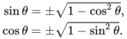

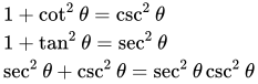
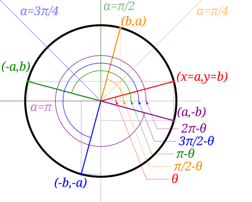


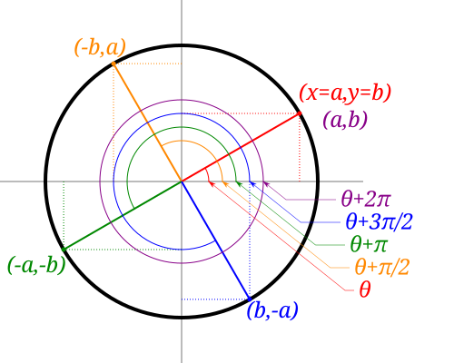


![{\displaystyle {\begin{aligned}\operatorname {sgn}(\sin \theta )=\operatorname {sgn}(\csc \theta )&={\begin{cases}+1&{\text{if}}\ \ 0<\theta <\pi \\-1&{\text{if}}\ \ {-\pi }} <\theta <0\\0&{\text{if}}\ \ \theta \in \{0,\pi \}\end{cases}}\\[5mu]\operatorname {sgn}(\cos \theta )=\operatorname {sgn}(\sec \theta )&={\begin{cases}+1&{\text{if}}\ \ {-{\tfrac {1}{2}}\pi }} <\theta <{\tfrac {1}{2}}\pi \\-1&{\text{if}}\ \ {-\pi }} <\theta <-{\tfrac {1}{2}}\pi \ \ {\text{or}}\ \ {\tfrac {1}{2}}\pi <\theta <\pi \\0&{\text{if}}\ \ \theta \in {\bigl \{}{-{\tfrac {1}{2}}\pi },{\tfrac {1}{2}}\pi {\bigr \}}\end{cases}}\\[5mu]\operatorname {sgn}(\tan \theta )=\operatorname {sgn}(\cot \theta )&={\begin{cases}+1&{\text{if}}\ \ {-\pi }} <\theta <-{\tfrac {1}{2}}\pi \ \ {\text{or}}\ \ 0<\theta <{\tfrac {1}{2}}\pi \\-1&{\text{if}}\ \ {-{\tfrac {1}{2}}\pi }}\ \ {\tfrac {1}{2}}\pi }}\theta <0\ \ {\text{または}}\ \ {\tfrac {1}{2}}\pi <\theta <\pi \\0&{\text{if}}\ \ \theta \in {\bigl \{}{-{\tfrac {1}{2}}\pi },0,{\tfrac {1}{2}}\pi ,\pi {\bigr \}}\end{cases}}\end{aligned}}}](https://wikimedia.org/api/rest_v1/media/math/render/svg/14cc79239a0fcdfb53b132d75a93474e9e6d5ba0)

![{\displaystyle ({-\pi },\pi ],}](https://wikimedia.org/api/rest_v1/media/math/render/svg/122328145a5f3a4162d21b4fbb5f4d1149932d2b)
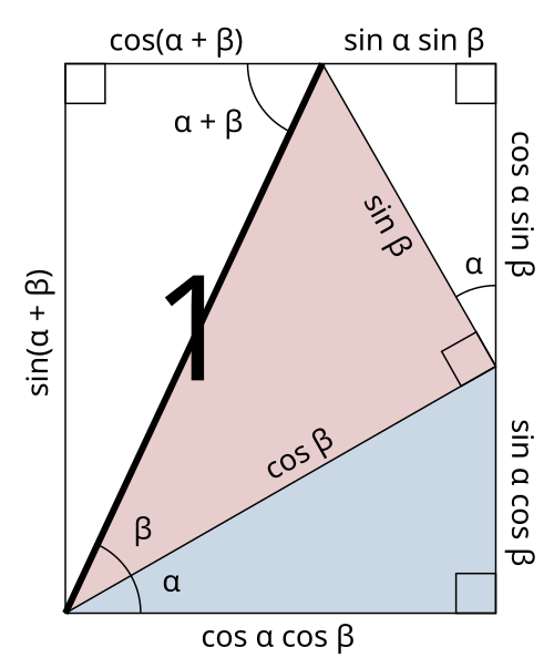
_and_cos(a-b).svg/500px-Diagram_showing_the_angle_difference_trigonometry_identities_for_sin(a-b)_and_cos(a-b).svg.png)


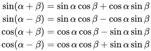





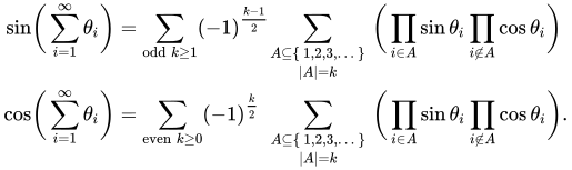







![{\displaystyle {\begin{aligned}e_{0}&=1\\[6pt]e_{1}&=\sum _{i}x_{i}&&=\sum _{i}\tan \theta _{i}\\[6pt]e_{2}&=\sum _{i<j}x_{i}x_{j}&&=\sum _{i<j}\tan \theta _{i}\tan \theta _{j}\\[6pt]e_{3}&=\sum _{i<j<k}x_{i}x_{j}x_{k}&&=\sum _{i<j<k}\tan \theta _{i}\tan \theta _{j}\tan \theta _{k}\\&\ \ \vdots &&\ \ \vdots \end{aligned}}}](https://wikimedia.org/api/rest_v1/media/math/render/svg/cb1927ae2be96f5156e18813a20486fdb0ff72f1)
![{\displaystyle {\begin{aligned}{\tan }{\Bigl (}\sum _{i}\theta _{i}{\Bigr )}&={\frac {{\sin }{\bigl (}\sum _{i}\theta _{i}{\bigr )}/\prod _{i}\cos \theta _{i}}{{\cos }{\bigl (}\sum _{i}\theta _{i}{\bigr )}/\prod _{i}\cos \theta _{i}}}\\[10pt]&={\frac {\displaystyle \sum _{{\text{odd}}\ k\geq 1}(-1)^{\frac {k-1}{2}}\sum _{\begin{smallmatrix}A\subseteq \{1,2,3,\dots \}\\\left|A\right|=k\end{smallmatrix}}\prod _{i\in A}\tan \theta _{i}}{\displaystyle \sum _{{\text{even}}\ k\geq 0}~(-1)^{\frac {k}{2}}~~\sum _{\begin{smallmatrix}A\subseteq \{1,2,3,\dots \}\\\left|A\right|=k\end{smallmatrix}}\prod _{i\in A}\tan \theta _{i}}}={\frac {e_{1}-e_{3}+e_{5}-\cdots }{e_{0}-e_{2}+e_{4}-\cdots }}\\[10pt]{\cot }{\Bigl (}\sum _{i}\theta _{i}{\Bigr )}&={\frac {e_{0}-e_{2}+e_{4}-\cdots }{e_{1}-e_{3}+e_{5}-\cdots }}\end{aligned}}}](https://wikimedia.org/api/rest_v1/media/math/render/svg/d02567417a5a013481366384787e518cd74c68be)
![{\displaystyle {\begin{aligned}\tan(\theta _{1}+\theta _{2})&={\frac {e_{1}}{e_{0}-e_{2}}}= {\frac {x_{1}+x_{2}}{1\ -\ x_{1}x_{2}}}={\frac {\tan \theta _{1}+\tan \theta _{2}}{1\ -\ \tan \theta _{1}\tan \theta _{2}}},\\[8pt]\tan(\theta _{1}+\theta _{2} +\theta _{3})&={\frac {e_{1}-e_{3}}{e_{0}-e_{2}}}={\frac {(x_{1}+x_{2}+x_{3})\ -\ (x_{1}x_{2}x_{3})}{1\ -\ (x_{1}x_{2}+x_{1}x_{3}+x_{2}x_{3}) }},\\[8pt]\tan(\theta _{1}+\theta _{2}+\theta _{3}+\theta _{4})&={\frac {e_{1}- e_{3}}{e_{0}-e_{2}+e_{4}}}\\[8pt]&={\frac {(x_{1}+x_{2}+x_{3}+x_ {4})\ -\ (x_{1}x_{2}x_{3}+x_{1}x_{2}x_{4}+x_{1}x_{3}x_{4}+x_{2}x_{3}x_{ 4})}{1\ -\ (x_{1}x_{2}+x_{1}x_{3}+x_{1}x_{4}+x_{2}x_{3}+x_{2} x_{4}+x_{3}x_{4})\ +\ (x_{1}x_{2}x_{3}x_{4})}},\end{aligned}}}](https://wikimedia.org/api/rest_v1/media/math/render/svg/4c9196b8ab5e0aef6cf7d7fec7d7546f2a6e7d2f)
![{\displaystyle {\begin{aligned}{\sec }{\Bigl (}\sum _{i}\theta _{i}{\Bigr )}&={\frac {\prod _{i}\sec \theta _{i}}{e_{0}-e_{2}+e_{4}-\cdots }}\\[8pt]{\csc }{\Bigl (}\sum _{i}\theta _{i}{\Bigr )}&={\frac {\prod _{i}\sec \theta _{i}}{e_{1}-e_{3}+e_{5}-\cdots }}\end{aligned}}}](https://wikimedia.org/api/rest_v1/media/math/render/svg/b24f2b169fbe11608507c63f5bb728e03b2b4957)


![{\displaystyle {\begin{aligned}\sec(\alpha +\beta +\gamma )&={\frac {\sec \alpha \sec \beta \sec \gamma }{1-\tan \alpha \tan \beta -\tan \alpha \tan \gamma -\tan \beta \tan \gamma }}\\[8pt]\csc(\alpha +\beta +\gamma )&={\frac {\sec \alpha \sec \beta \sec \gamma }{\tan \alpha +\tan \beta +\tan \gamma -\tan \alpha \tan \beta \tan \gamma }}.\end{aligned}}}](https://wikimedia.org/api/rest_v1/media/math/render/svg/e082e69aab7a9c782f590f3a93262ba3101899b7)


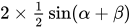








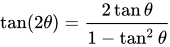






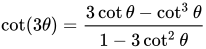
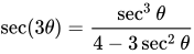
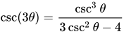




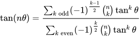


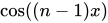
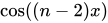





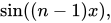
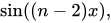





![{\displaystyle {\begin{aligned}\sin {\frac {\theta }{2}}&=\operatorname {sgn} \left(\sin {\frac {\theta }{2}}\right){\sqrt {\frac {1-\cos \theta }{2}}}\\[3pt]\cos {\frac {\theta }{2}}&=\operatorname {sgn} \left(\cos {\frac {\theta }{2}}\right){\sqrt {\frac {1+\cos \theta }{2}}}\\[3pt]\tan {\frac {\theta }{2}}&={\frac {1-\cos \theta }{\sin \theta }}={\frac {\sin \theta }{1+\cos \theta }}=\csc \theta -\cot \theta ={\frac {\tan \theta }{1+\sec {\theta }}}\\[6mu]&=\operatorname {sgn}(\sin \theta ){\sqrt {\frac {1-\cos \theta }{1+\cos \theta }}}={\frac {-1+\operatorname {sgn}(\cos \theta ){\sqrt {1+\tan ^{2}\theta }}}{\tan \theta }}\\[3pt]\cot {\frac {\theta }{2}}&={\frac {1+\cos \theta }{\sin \theta }}={\frac {\sin \theta }{1-\cos \theta }}=\csc \theta +\cot \theta =\operatorname {sgn}(\sin \theta ){\sqrt {\frac {1+\cos \theta }{1-\cos \theta }}}\\\sec {\frac {\theta }{2}}&=\operatorname {sgn} \left(\cos {\frac {\theta }{2}}\right){\sqrt {\frac {2}{1+\cos \theta }}}\\\csc {\frac {\theta }{2}}&=\operatorname {sgn} \left(\sin {\frac {\theta }{2}}\right){\sqrt {\frac {2}{1-\cos \theta }}}\\\end{aligned}}}](https://wikimedia.org/api/rest_v1/media/math/render/svg/d53d104c73c4b28f1dd7bfa5d2b0c7207c68cd87)
![{\displaystyle {\begin{aligned}\tan {\frac {\eta \pm \theta }{2}}&={\frac {\sin \eta \pm \sin \theta }{\cos \eta +\cos \theta }}\\[3pt]\tan \left({\frac {\theta }{2}}+{\frac {\pi }{4}}\right)&=\sec \theta +\tan \theta \\[3pt]{\sqrt {\frac {1-\sin \theta }{1+\sin \theta }}}&={\frac {\left|1-\tan {\frac {\theta }{2}}\right|}{\left|1+\tan {\frac {\theta }{2}}\right|}}\end{aligned}}}](https://wikimedia.org/api/rest_v1/media/math/render/svg/639270245e163f1afa8682ac8aa12086db43dce1)





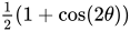












![{\displaystyle {\begin{aligned}\cos \theta \,\cos \varphi &={\tfrac {1}{2}}{\bigl (}\!\!~\cos(\theta -\varphi ) +\cos(\theta +\varphi ){\bigr )}\\[3mu]\sin \theta \,\sin \varphi &={\tfrac {1}{2}}{\bigl (}\!\!~\cos(\theta -\varphi )-\cos(\theta +\varphi ){\bigr )}\\[3mu]\sin \theta \,\cos \varphi &={\tfrac {1}{2}}{\bigl (}\!\!~\sin(\theta +\varphi )+\sin(\theta -\varphi ){\bigr )}\\[3mu]\cos \theta \,\sin \varphi &={\tfrac {1}{2}}{\bigl (}\!\!~\sin(\theta +\ varphi )-\sin(\theta -\varphi ){\bigr )}\end{aligned}}}](https://wikimedia.org/api/rest_v1/media/math/render/svg/aa5a52add0153b90bd4863677fe0eab2f1700561)


![{\displaystyle {\begin{aligned}\prod _{k=1}^{n}\cos \theta _{k}&={\frac {1}{2^{n}}}\sum _{e\in S}\cos(e_{1}\theta _{1}+\cdots +e_{n}\theta _{n})\\[6pt]&{\text{where }}e=(e_{1},\ldots ,e_{n})\in S=\{1,-1\}^{n}\end{aligned}}}](https://wikimedia.org/api/rest_v1/media/math/render/svg/ce2126a8ded0d0c92cf2bc4e9386c34430513c4b)
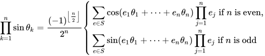


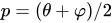
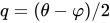






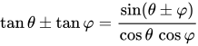

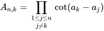




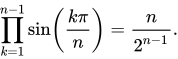

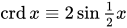
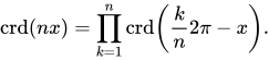



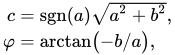


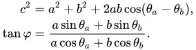

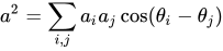
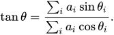
![{\displaystyle {\begin{aligned}\sum _{k=0}^{n}\sin k\theta &={\frac {\cos {\tfrac {1}{2}}\theta -\cos \left(\left(n+{\tfrac {1}{2}}\right)\theta \right)}{2\sin {\tfrac {1}{2}}\theta }}\\[5pt]\sum _{k=0}^{n}\cos k\theta &={\frac {\sin {\tfrac {1}{2}}\theta +\sin \left(\left(n+{\tfrac {1}{2}}\right)\theta \right)}{2\sin {\tfrac {1}{2}}\theta }}\end{aligned}}}](https://wikimedia.org/api/rest_v1/media/math/render/svg/c850aa2dd7cc306d87d5d68d5802cab64f8572a0)


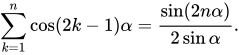


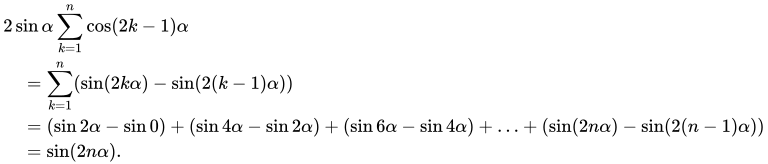


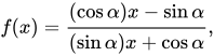
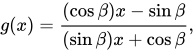





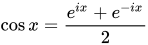
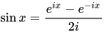



![{\displaystyle {\begin{aligned}\sin x&=x\prod _{n=1}^{\infty }\left(1-{\frac {x^{2}}{\pi ^{2}n^{2}}}\right),&\cos x&=\prod _{n=1}^{\infty }\left(1-{\frac {x^{2}}{\pi ^{2}\left(n-{\frac {1}{2}}\right)\!{\vphantom {)}}^{2}}}\right),\\[10mu]\sinh x&=x\prod _{n=1}^{\infty }\left(1+{\frac {x^{2}}{\pi ^{2}n^{2}}}\right),&\cosh x&=\prod _{n=1}^{\infty }\left(1+{\frac {x^{2}}{\pi ^{2}\left(n-{\frac {1}{2}}\right)\!{\vphantom {)}}^{2}}}\right).\end{aligned}}}](https://wikimedia.org/api/rest_v1/media/math/render/svg/6d43e1176a38b1e6b653837eb782ae79735783ac)
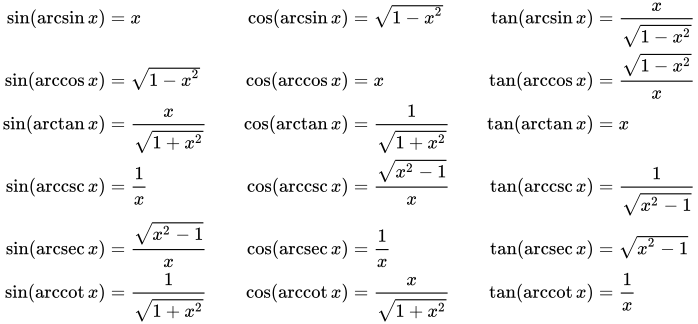

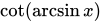

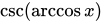
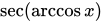


![{\displaystyle {\begin{alignedat}{9}{\frac {\pi }{2}}~&=~\arcsin(x)&&+\arccos(x)~&&=~\arctan(r)&&+\operatorname {arccot}(r)~&&=~\operatorname {arcsec}(s)&&+\operatorname {arccsc}(s)\\[0.4ex]\pi ~&=~\arccos(x)&&+\arccos(-x)~&&=~\operatorname {arccot}(r)&&+\operatorname {arccot}(-r)~&&=~\operatorname {arcsec}(s)&&+\operatorname {arcsec}(-s)\\[0.4ex]0~&=~\arcsin(x)&&+\arcsin(-x)~&&=~\arctan(r)&&+\arctan(-r)~&&=~\operatorname {arccsc}(s)&&+\operatorname {arccsc}(-s)\\[1.0ex]\end{alignedat}}}](https://wikimedia.org/api/rest_v1/media/math/render/svg/839db041f421b4af5890106450e2b4d3e9e183d4)