NBGの公理化
外延性とペアリングの定義と公理 セットとは、少なくとも1つのクラスに属するクラスのことです。A {\displaystyle A} ∃ C ( A ∈ C ) {\displaystyle \exists C(A\in C)} A {\displaystyle A} ∀ C ( A ∉ C ) {\displaystyle \forall C(A\notin C)} 12 ]したがって、すべてのクラス は
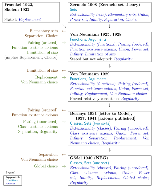
ゲーデルは、大文字の変数はクラスを、小文字の変数は集合を表すという慣習を導入した。[ 9 ] ゲーデルはまた、すべての集合のクラスで定義された関数や関係 など、特定のクラスを表すために大文字で始まる名前を使用した。この記事ではゲーデルの慣習を採用する。これにより、次のように記述できる。
∃ x ϕ ( x ) {\displaystyle \exists x\,\phi (x)} ∃ x ( ∃ C ( x ∈ C ) ∧ ϕ ( x ) ) {\displaystyle \exists x{\bigl (}\exists C(x\in C)\land \phi (x){\bigr )}} ∀ x ϕ ( x ) {\displaystyle \forall x\,\phi (x)} ∀ x ( ∃ C ( x ∈ C ) ⟹ ϕ ( x ) ) \displaystyle \forall x{\bigl (}\exists C(x\in C)\implies \phi (x){\bigr )}} クラス存在定理の証明には、以下の公理と定義が必要となる。
外延性の公理。2 つのクラスが同じ要素を持つならば、それらは同一である。
∀ A ∀ B [ ∀ x ( x ∈ A ⟺ x ∈ B ) ⟹ A = B ] {\displaystyle \forall A\,\forall B\,[\forall x(x\in A\iff x\in B)\implies A=B]} [ 13 ] この公理は、ZFCの外延性公理を クラスに一般化したものである。
ペアリングの 。 x {\displaystyle x} y {\displaystyle y} p {\displaystyle p} x {\displaystyle x} y {\displaystyle y}
∀ x ∀ y ∃ p ∀ z [ z ∈ p ⟺ ( z = x ∨ z = y ) ] {\displaystyle \forall x\,\forall y\,\exists p\,\forall z\,[z\in p\iff (z=x\,\lor \,z=y)]} [ 14 ] ZFCと同様に、外延性 の公理は集合の一意性を意味する。p {\displaystyle p} { x 、 y } 。 {\displaystyle \{x,y\}.}
順序対は 次のように定義されます。
( x 、 y ) = { { x } 、 { x 、 y } } {\displaystyle (x,y)=\{\{x\},\{x,y\}\}} タプルは順序対を用いて帰納的に 定義される。
( x 1 ) = x 1 、 {\displaystyle (x_{1})=x_{1},} のために n > 1 : ( x 1 、 … 、 x n − 1 、 x n ) = ( ( x 1 、 … 、 x n − 1 ) 、 x n ) 。 {\displaystyle {\text{For }}n>1\!:(x_{1},\ldots ,x_{n-1},x_{n})=((x_{1},\ldots ,x_{n-1}),x_{n}).} [ c ]
クラス存在公理と規則性公理 クラス存在公理を用いてクラス存在定理を証明する:すべての式に対してn {\displaystyle n} 集合のみを量化する自由 集合変数のクラスが存在するn {\displaystyle n} 関数 である 2 つのクラスから始めて、複合関数 を構築します。この例は、クラス存在定理を証明するために必要な手法を示しており、それによって必要なクラス存在公理が得られます。
クラス存在公理は、言語プリミティブを扱う公理とタプルを扱う公理の2つのグループに分けられます。最初のグループには4つの公理があり、2番目のグループには3つの公理があります。[ d ]
言語プリミティブを扱うための公理:
メンバーシップ。 クラスが存在するE {\displaystyle E}
∃ E ∀ x ∀ y [ ( x 、 y ) ∈ E ⟺ x ∈ y ] {\displaystyle \exists E\,\forall x\,\forall y\,[(x,y)\in E\iff x\in y]\!} [ 18 ] 交差(結合)。 任意の2つのクラスについてA {\displaystyle A} B {\displaystyle B} C {\displaystyle C} A {\displaystyle A} B {\displaystyle B}
∀ A ∀ B ∃ C ∀ x [ x ∈ C ⟺ ( x ∈ A ∧ x ∈ B ) ] {\displaystyle \forall A\,\forall B\,\exists C\,\forall x\,[x\in C\iff (x\in A\,\land \,x\in B)]} [ 19 ] 補数 (否定)。A {\displaystyle A} B {\displaystyle B} A {\displaystyle A}
∀ A ∃ B ∀ x [ x ∈ B ⟺ ¬ ( x ∈ A ) ] {\displaystyle \forall A\,\exists B\,\forall x\,[x\in B\iff \neg (x\in A)]} [ 20 ] ドメイン(存在量化子)。 任意のクラスに対してA {\displaystyle A} B {\displaystyle B} A {\displaystyle A}
∀ A ∃ B ∀ x [ x ∈ B ⟺ ∃ y ( ( x 、 y ) ∈ A ) ] {\displaystyle \forall A\,\exists B\,\forall x\,[x\in B\iff \exists y((x,y)\in A)]} [ 21 ] 外延性の公理により、クラスC {\displaystyle C} B {\displaystyle B} A ∩ B 、 {\displaystyle A\cap B,} ∁ ( A ) 、 {\displaystyle \complement (A),} D o m ( A ) 、 {\displaystyle Dom(A),} [ e ]
E 。 {\displaystyle E.} E ∩ ∁ ( E ) {\displaystyle E\cap \complement (E)} ∅ 。 {\displaystyle \emptyset .} ∅ {\displaystyle \emptyset } V {\displaystyle V} M ( A ) {\displaystyle M(A)} ∃ C ( A ∈ C ) {\displaystyle \exists C(A\in C)} A ∈ V {\displaystyle A\in V}
タプルを扱うための公理:
製品 V {\displaystyle V} も A {\displaystyle A} B {\displaystyle B} A {\displaystyle A}
∀ A ∃ B ∀ u [ u ∈ B ⟺ ∃ x ∃ y ( u = ( x 、 y ) ∧ x ∈ A ) ] {\displaystyle \forall A\,\exists B\,\forall u\,[u\in B\iff \exists x\,\exists y\,(u=(x,y)\land x\in A)]} [ 23 ] 円順列 。A {\displaystyle A} B {\displaystyle B} タプル は、円順列を適用することによって得られる。( y 、 z 、 x ) ↦ ( x 、 y 、 z ) {\displaystyle (y,z,x)\mapsto (x,y,z)} タプル へA {\displaystyle A}
∀ A ∃ B ∀ x ∀ y ∀ z [ ( x 、 y 、 z ) ∈ B ⟺ ( y 、 z 、 x ) ∈ A ] {\displaystyle \forall A\,\exists B\,\forall x\,\forall y\,\forall z\,[(x,y,z)\in B\iff (y,z,x)\in A]} [ 24 ] 転置 。A {\displaystyle A} B {\displaystyle B} タプルは、 の 3 タプルの最後の 2 つのコンポーネントを転置することによって得られる。A {\displaystyle A}
∀ A ∃ B ∀ x ∀ y ∀ z [ ( x 、 y 、 z ) ∈ B ⟺ ( x 、 z 、 y ) ∈ A ] {\displaystyle \forall A\,\exists B\,\forall x\,\forall y\,\forall z\,[(x,y,z)\in B\iff (x,z,y)\in A]} [ 25 ] 外延性により、V {\displaystyle V} A × V 。 {\displaystyle A\times V.} V n {\displaystyle V^{n}} n {\displaystyle n} V 1 = V {\displaystyle V^{1}=V} V n + 1 = V n × V 。 {\displaystyle V^{n+1}=V^{n}\times V.\,} A {\displaystyle A} A ∩ V n {\displaystyle A\cap V^{n}} n {\displaystyle n} タプル A 。 {\displaystyle A.} E {\displaystyle E} E ∩ V 2 {\displaystyle E\cap V^{2}} E {\displaystyle E}
円順列と転置の公理は、クラスの 3 タプルのみ を指定するため、一意のクラスの存在を意味しません。B 。 {\displaystyle B.} 、 これらの公理は、n {\displaystyle n} タプル n ≥ 4 {\displaystyle n\geq 4} ( x 1 、 … 、 x n − 2 、 x n − 1 、 x n ) = ( ( x 1 、 … 、 x n − 2 ) 、 x n − 1 、 x n ) 。 {\displaystyle (x_{1},\ldots ,x_{n-2},x_{n-1},x_{n})=((x_{1},\ldots ,x_{n-2}),x_{n-1},x_{n}).}
タプル補題 —
∀ A ∃ B 1 ∀ x ∀ y ∀ z [ ( z 、 x 、 y ) ∈ B 1 ⟺ ( x 、 y ) ∈ A ] {\displaystyle \forall A\,\exists B_{1}\,\forall x\,\forall y\,\forall z\,[(z,x,y)\in B_{1}\iff (x,y)\in A]} ∀ A ∃ B 2 ∀ x ∀ y ∀ z [ ( x 、 z 、 y ) ∈ B 2 ⟺ ( x 、 y ) ∈ A ] {\displaystyle \forall A\,\exists B_{2}\,\forall x\,\forall y\,\forall z\,[(x,z,y)\in B_{2}\iff (x,y)\in A]} ∀ A ∃ B 3 ∀ x ∀ y ∀ z [ ( x 、 y 、 z ) ∈ B 3 ⟺ ( x 、 y ) ∈ A ] {\displaystyle \forall A\,\exists B_{3}\,\forall x\,\forall y\,\forall z\,[(x,y,z)\in B_{3}\iff (x,y)\in A]} ∀ A ∃ B 4 ∀ x ∀ y ∀ z [ ( y 、 x ) ∈ B 4 ⟺ ( x 、 y ) ∈ A ] {\displaystyle \forall A\,\exists B_{4}\,\forall x\,\forall y\,\forall z\,[(y,x)\in B_{4}\iff (x,y)\in A]} 証拠 クラスB 3 {\displaystyle B_{3}} V {\displaystyle V} A {\displaystyle A} B 3 。 {\displaystyle B_{3}.} クラスB 2 {\displaystyle B_{2}} B 3 {\displaystyle B_{3}} B 2 。 {\displaystyle B_{2}.} クラスB 1 {\displaystyle B_{1}} B 3 {\displaystyle B_{3}} B 1 。 {\displaystyle B_{1}.} クラスB 4 {\displaystyle B_{4}} B 2 {\displaystyle B_{2}} B 4 。 {\displaystyle B_{4}.} クラス存在定理を証明するには、もう1つの公理、すなわち正則性の公理 が必要です。空クラスの存在は既に証明されているので、この公理の通常の記述を以下に示します。[ f ]
正則性の公理 。∀ 1 [ 1 ≠ ∅ ⟹ ∃ u ( u ∈ 1 ∧ u ∩ 1 = ∅ ) ] 。 {\displaystyle \forall a\,[a\neq \emptyset \implies \exists u(u\in a\land u\cap a=\emptyset )].}
この公理は、集合がそれ自身に属することはできないことを示唆している。x ∈ x {\displaystyle x\in x} 1 = { x } 。 {\displaystyle a=\{x\}.} x ∩ 1 ≠ ∅ {\displaystyle x\cap a\neq \emptyset } x ∈ x ∩ 1 。 {\displaystyle x\in x\cap a.} x {\displaystyle x} 1 。 {\displaystyle a.} x ∉ x 。 {\displaystyle x\notin x.} ⋯ ∈ x n + 1 ∈ x n ∈ ⋯ ∈ x 1 ∈ x 0 。 {\displaystyle \cdots \in x_{n+1}\in x_{n}\in \cdots \in x_{1}\in x_{0}.}
ゲーデルは、1938年に行われた講義に基づいて1940年に発表したモノグラフの中で、集合ではなくクラスの正則性を述べた。 [ 26 ] [ 27 ]
クラス存在定理
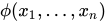
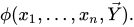
クラス存在定理 — とϕ ( x 1 、 … 、 x n 、 Y 1 、 … 、 Y m ) {\displaystyle \phi (x_{1},\dots ,x_{n},Y_{1},\dots ,Y_{m})} 自由変数 を含まない式であること。x 1 、 … 、 x n 、 Y 1 、 … 、 Y m {\displaystyle x_{1},\dots ,x_{n},Y_{1},\dots ,Y_{m}} Y 1 、 … 、 Y m {\displaystyle Y_{1},\dots ,Y_{m}} A {\displaystyle A} n {\displaystyle n} ∀ x 1 ⋯ ∀ x n [ ( x 1 、 … 、 x n ) ∈ A ⟺ ϕ ( x 1 、 … 、 x n 、 Y 1 、 … 、 Y m ) ] 。 {\displaystyle \forall x_{1}\cdots \,\forall x_{n}[(x_{1},\dots ,x_{n})\in A\iff \phi (x_{1},\dots ,x_{n},Y_{1},\dots ,Y_{m})].} A {\displaystyle A} { ( x 1 、 … 、 x n ) : ϕ ( x 1 、 … 、 x n 、 Y 1 、 … 、 Y m ) } 。 {\displaystyle \{(x_{1},\dots ,x_{n}):\phi (x_{1},\dots ,x_{n},Y_{1},\dots ,Y_{m})\}.} [ g ]
この定理の証明は2つのステップで行います。
変換ルールは、与えられた式を変換するために使用されます。ϕ {\displaystyle \phi } 証明の帰納 部分を簡略化する同等の 式に変換します。たとえば、変換後の式に含まれる論理記号は、¬ {\displaystyle \neg } ∧ {\displaystyle \land } ∃ {\displaystyle \exists } クラス存在定理は、変換された式に対して帰納的に証明される。変換された式の構造に導かれて、クラス存在公理を使用して、一意のクラスを生成する。n {\displaystyle n} タプル。 変換ルール。 以下のルール1と2では、Δ {\displaystyle \Delta } Γ {\displaystyle \Gamma } ∈ {\displaystyle \in } 私 {\displaystyle i} z 私 {\displaystyle z_{i}} ¬ {\displaystyle \neg } ∧ {\displaystyle \land } ∃ {\displaystyle \exists } ∈ {\displaystyle \in } Y k {\displaystyle Y_{k}} Y k {\displaystyle Y_{k}} ∈ {\displaystyle \in }
Y k ∈ Γ {\displaystyle \,Y_{k}\in \Gamma } ∃ z 私 ( z 私 = Y k ∧ z 私 ∈ Γ ) 。 {\displaystyle \exists z_{i}(z_{i}=Y_{k}\,\land \,z_{i}\in \Gamma ).} 外延性は変換するために用いられるΔ = Γ {\displaystyle \Delta =\Gamma } ∀ z 私 ( z 私 ∈ Δ ⟺ z 私 ∈ Γ ) 。 {\displaystyle \forall z_{i}(z_{i}\in \Delta \iff z_{i}\in \Gamma ).} 論理的恒等式は、以下の部分式を変換するために使用されます。∨ 、 ⟹ 、 ⟺ 、 {\displaystyle \lor ,\implies ,\iff ,} ∀ {\displaystyle \forall } ¬ 、 ∧ 、 {\displaystyle \neg ,\land ,} ∃ 。 {\displaystyle \exists .} 変換ルール:束縛変数 。 例1 の合成関数式を考え、その自由集合変数を次のように置き換えます。x 1 {\displaystyle x_{1}} x 2 {\displaystyle x_{2}} ∃ t [ ( x 1 、 t ) ∈ F ∧ ( t 、 x 2 ) ∈ G ] 。 {\displaystyle \exists t[(x_{1},t)\in F\,\land \,(t,x_{2})\in G].} ∃ t {\displaystyle \exists t} ( x 1 、 t ) ∈ F ∧ ( t 、 x 2 ) ∈ G 。 {\displaystyle (x_{1},t)\in F\land (t,x_{2})\in G.} しかし、クラス存在定理は添え字付き変数に対して述べられているため、この式は帰納法の仮説 が期待する形式とは異なっている。この問題は変数を置き換えることで解決される。t {\displaystyle t} x 3 。 {\displaystyle x_{3}.}
式に自由セット変数が含まれない場合、x 1 、 … 、 x n 、 {\displaystyle x_{1},\dots ,x_{n},} q {\displaystyle q} x n + q {\displaystyle x_{n+q}} ( 量化子)のネスト深度を持つ q {\displaystyle q}
クラス存在定理の証明。 証明は、与えられた式に変換規則を適用して変換後の式を生成することから始まります。この式は与えられた式と等価であるため、変換後の式に対するクラス存在定理を証明することで証明が完了します。
変換された式のクラス存在定理の証明 証明では以下の補題が用いられる。
証拠:
もし私 = 1 、 {\displaystyle i=1,} P 1 = P 。 {\displaystyle P_{1}=P.}
さもないと、私 > 1 、 {\displaystyle i>1,} x 私 : {\displaystyle x_{i}{\text{:}}} タプル補題 のステートメント1を適用するP {\displaystyle P} z = ( x 1 、 … 、 x 私 − 1 ) 。 {\displaystyle z=(x_{1},\dots ,x_{i-1}).} P 1 {\displaystyle P_{1}} ( 私 + 1 ) {\displaystyle (i+1)} ( ( x 1 、 … 、 x 私 − 1 ) 、 x 私 、 x j ) = ( x 1 、 … 、 x 私 − 1 、 x 私 、 x j ) {\displaystyle ((x_{1},\dots ,x_{i-1}),x_{i},x_{j})=(x_{1},\dots ,x_{i-1},x_{i},x_{j})} R ( x 私 、 x j ) 。 {\displaystyle R(x_{i},x_{j}).} もしj = 私 + 1 、 {\displaystyle j=i+1,} P 2 = P 1 。 {\displaystyle P_{2}=P_{1}.}
さもないと、j > 私 + 1 、 {\displaystyle j>i+1,} x 私 {\displaystyle x_{i}} x j : {\displaystyle x_{j}{\text{:}}} x 私 + 1 、 … 、 x j − 1 {\displaystyle x_{i+1},\dots ,x_{j-1}} P 2 {\displaystyle P_{2}} j {\displaystyle j} ( ( ( ⋯ ( ( x 1 、 … 、 x 私 ) 、 x 私 + 1 ) 、 ⋯ ) 、 x j − 1 ) 、 x j ) = ( x 1 、 … 、 x j ) {\displaystyle (((\cdots ((x_{1},\dots ,x_{i}),x_{i+1}),\cdots ),x_{j-1}),x_{j})=(x_{1},\dots ,x_{j})} R ( x 私 、 x j ) 。 {\displaystyle R(x_{i},x_{j}).} もしj = n 、 {\displaystyle j=n,} P 3 = P 2 。 {\displaystyle P_{3}=P_{2}.}
さもないと、j < n 、 {\displaystyle j<n,} x j : {\displaystyle x_{j}{\text{:}}} x j + 1 、 … 、 x n {\displaystyle x_{j+1},\dots ,x_{n}} P 3 {\displaystyle P_{3}} n {\displaystyle n} ( ( ⋯ ( ( x 1 、 … 、 x j ) 、 x j + 1 ) 、 ⋯ ) 、 x n ) = ( x 1 、 … 、 x n ) {\displaystyle ((\cdots ((x_{1},\dots ,x_{j}),x_{j+1}),\cdots ),x_{n})=(x_{1},\dots ,x_{n})} R ( x 私 、 x j ) 。 {\displaystyle R(x_{i},x_{j}).} させてQ = P 3 ∩ V n 。 {\displaystyle Q=P_{3}\cap V^{n}.} Q {\displaystyle Q} n {\displaystyle n} R ( x 私 、 x j ) 。 {\displaystyle R(x_{i},x_{j}).} 変換された式のクラス存在定理 — としますϕ ( x 1 、 … 、 x n 、 Y 1 、 … 、 Y m ) {\displaystyle \phi (x_{1},\ldots ,x_{n},Y_{1},\ldots ,Y_{m})}
以外の自由変数は含まれていません。x 1 、 … 、 x n 、 Y 1 、 … 、 Y m {\displaystyle x_{1},\ldots ,x_{n},Y_{1},\ldots ,Y_{m}} のみを含む∈ {\displaystyle \in } ¬ {\displaystyle \neg } ∧ {\displaystyle \land } ∃ {\displaystyle \exists } Y k {\displaystyle Y_{k}} Y k {\displaystyle Y_{k}} ∈ {\displaystyle \in } セット変数のみを定量化しますx n + q {\displaystyle x_{n+q}} q {\displaystyle q} そしてすべてのY 1 、 … 、 Y m {\displaystyle Y_{1},\dots ,Y_{m}} A {\displaystyle A} n {\displaystyle n} ∀ x 1 ⋯ ∀ x n [ ( x 1 、 … 、 x n ) ∈ A ⟺ ϕ ( x 1 、 … 、 x n 、 Y 1 、 … 、 Y m ) ] 。 {\displaystyle \forall x_{1}\cdots \,\forall x_{n}[(x_{1},\ldots ,x_{n})\in A\iff \phi (x_{1},\ldots ,x_{n},Y_{1},\ldots ,Y_{m})].}
証明:基本ステップ:ϕ {\displaystyle \phi } ϕ {\displaystyle \phi } x 私 ∈ x j {\displaystyle x_{i}\in x_{j}} x 私 ∈ Y k 。 {\displaystyle x_{i}\in Y_{k}.}
ケース1:もしϕ {\displaystyle \phi } x 私 ∈ x j {\displaystyle x_{i}\in x_{j}} E 私 、 j 、 n = { ( x 1 、 … 、 x n ) : x 私 ∈ x j } 、 {\displaystyle E_{i,j,n}=\{(x_{1},\ldots ,x_{n}):x_{i}\in x_{j}\},} n {\displaystyle n} x 私 ∈ x j 。 {\displaystyle x_{i}\in x_{j}.}
ケースa:ϕ {\displaystyle \phi } x 私 ∈ x j {\displaystyle x_{i}\in x_{j}} 私 < j 。 {\displaystyle i<j.} P {\displaystyle P} ( x 私 、 x j ) {\displaystyle (x_{i},x_{j})} x 私 ∈ x j 。 {\displaystyle x_{i}\in x_{j}.} P {\displaystyle P} E 私 、 j 、 n = { ( x 1 、 … 、 x n ) : x 私 ∈ x j } 。 {\displaystyle E_{i,j,n}=\{(x_{1},\ldots ,x_{n}):x_{i}\in x_{j}\}.}
ケースb:ϕ {\displaystyle \phi } x 私 ∈ x j {\displaystyle x_{i}\in x_{j}} 私 > j 。 {\displaystyle i>j.} P {\displaystyle P} ( x 私 、 x j ) {\displaystyle (x_{i},x_{j})} x 私 ∈ x j 。 {\displaystyle x_{i}\in x_{j}.} P {\displaystyle P} P ′ {\displaystyle P'} ( x j 、 x 私 ) {\displaystyle (x_{j},x_{i})} x 私 ∈ x j 。 {\displaystyle x_{i}\in x_{j}.} P ′ {\displaystyle P'} E 私 、 j 、 n = { ( x 1 、 … 、 x n ) : x 私 ∈ x j } 。 {\displaystyle E_{i,j,n}=\{(x_{1},\ldots ,x_{n}):x_{i}\in x_{j}\}.}
ケースc:ϕ {\displaystyle \phi } x 私 ∈ x j {\displaystyle x_{i}\in x_{j}} 私 = j 。 {\displaystyle i=j.} 正則性の公理 により偽であるため、n {\displaystyle n} E 私 、 j 、 n = ∅ 。 {\displaystyle E_{i,j,n}=\emptyset .}
ケース2:もしϕ {\displaystyle \phi } x 私 ∈ Y k {\displaystyle x_{i}\in Y_{k}} E 私 、 Y k 、 n = { ( x 1 、 … 、 x n ) : x 私 ∈ Y k } 、 {\displaystyle E_{i,Y_{k},n}=\{(x_{1},\ldots ,x_{n}):x_{i}\in Y_{k}\},} n {\displaystyle n} x 私 ∈ Y k 。 {\displaystyle x_{i}\in Y_{k}.}
ケースa:ϕ {\displaystyle \phi } x 私 ∈ Y k {\displaystyle x_{i}\in Y_{k}} 私 < n 。 {\displaystyle i<n.} V {\displaystyle V} Y k {\displaystyle Y_{k}} P = Y k × V = { ( x 私 、 x 私 + 1 ) : x 私 ∈ Y k } 。 {\displaystyle P=Y_{k}\times V=\{(x_{i},x_{i+1}):x_{i}\in Y_{k}\}.} P {\displaystyle P} E 私 、 Y k 、 n = { ( x 1 、 … 、 x n ) : x 私 ∈ Y k } 。 {\displaystyle E_{i,Y_{k},n}=\{(x_{1},\ldots ,x_{n}):x_{i}\in Y_{k}\}.}
ケースb:ϕ {\displaystyle \phi } x 私 ∈ Y k {\displaystyle x_{i}\in Y_{k}} 私 = n > 1. {\displaystyle i=n>1.} V {\displaystyle V} Y k {\displaystyle Y_{k}} P = Y k × V = { ( x 私 、 x 私 − 1 ) : x 私 ∈ Y k } 。 {\displaystyle P=Y_{k}\times V=\{(x_{i},x_{i-1}):x_{i}\in Y_{k}\}.} P {\displaystyle P} P ′ = V × Y k = { ( x 私 − 1 、 x 私 ) : x 私 ∈ Y k } 。 {\displaystyle P'=V\times Y_{k}=\{(x_{i-1},x_{i}):x_{i}\in Y_{k}\}.} P ′ {\displaystyle P'} E 私 、 Y k 、 n = { ( x 1 、 … 、 x n ) : x 私 ∈ Y k } 。 {\displaystyle E_{i,Y_{k},n}=\{(x_{1},\ldots ,x_{n}):x_{i}\in Y_{k}\}.}
ケースc:ϕ {\displaystyle \phi } x 私 ∈ Y k {\displaystyle x_{i}\in Y_{k}} 私 = n = 1. {\displaystyle i=n=1.} E 私 、 Y k 、 n = Y k 。 {\displaystyle E_{i,Y_{k},n}=Y_{k}.}
帰納的ステップ:ϕ {\displaystyle \phi } k {\displaystyle k} k > 0 {\displaystyle k>0} ψ {\displaystyle \psi } k {\displaystyle k} ϕ {\displaystyle \phi } k {\displaystyle k} Y 1 、 … 、 Y m {\displaystyle Y_{1},\dots ,Y_{m}} Y → {\displaystyle {\vec {Y}}} ϕ ( x 1 、 … 、 x n 、 Y 1 、 … 、 Y m ) {\displaystyle \phi (x_{1},\dots ,x_{n},Y_{1},\dots ,Y_{m})} ϕ ( x 1 、 … 、 x n 、 Y → ) 。 {\displaystyle \phi (x_{1},\dots ,x_{n},{\vec {Y}}).}
ケース1:ϕ ( x 1 、 … 、 x n 、 Y → ) = ¬ ψ ( x 1 、 … 、 x n 、 Y → ) 。 {\displaystyle \phi (x_{1},\ldots ,x_{n},{\vec {Y}})=\neg \psi (x_{1},\ldots ,x_{n},{\vec {Y}}).} ψ {\displaystyle \psi } k − 1 {\displaystyle k-1} A {\displaystyle A} n {\displaystyle n} ( x 1 、 … 、 x n ) ∈ A ⟺ ψ ( x 1 、 … 、 x n 、 Y → ) 。 {\displaystyle \quad (x_{1},\ldots ,x_{n})\in A\iff \psi (x_{1},\ldots ,x_{n},{\vec {Y}}).} ∁ ( A ) {\displaystyle \complement (A)} ∀ u [ u ∈ ∁ ( A ) ⟺ ¬ ( u ∈ A ) ] 。 {\displaystyle \forall u\,[u\in \complement (A)\iff \neg (u\in A)].} ∁ ( A ) {\displaystyle \complement (A)} n {\displaystyle n} n > 1. {\displaystyle n>1.} ∁ V n ( A ) = {\displaystyle \complement _{V^{n}}(A)=\,} ∁ ( A ) ∩ V n = {\displaystyle \complement (A)\cap V^{n}=\,} V n ∖ A 、 {\displaystyle V^{n}\setminus A,} V n {\displaystyle V^{n}} n {\displaystyle n} [ e ] ∁ V n A {\displaystyle \complement _{V^{n}}A} n {\displaystyle n} ( x 1 、 … 、 x n ) ∈ ∁ V n ( A ) ⟺ ¬ [ ( x 1 、 … 、 x n ) ∈ A ] ⟺ ¬ ψ ( x 1 、 … 、 x n 、 Y → ) ⟺ ϕ ( x 1 、 … 、 x n 、 Y → ) 。 {\displaystyle {\begin{alignedat}{2}\quad &(x_{1},\ldots ,x_{n})\in \complement _{V^{n}}(A)&&\iff \neg [(x_{1},\ldots ,x_{n})\in A]\\&&&\iff \neg \psi (x_{1},\ldots ,x_{n},{\vec {Y}})\\&&&\iff \phi (x_{1},\ldots ,x_{n},{\vec {Y}}).\end{alignedat}}}
ケース2:ϕ ( x 1 、 … 、 x n 、 Y → ) = ψ 1 ( x 1 、 … 、 x n 、 Y → ) ∧ ψ 2 ( x 1 、 … 、 x n 、 Y → ) 。 {\displaystyle \phi (x_{1},\ldots ,x_{n},{\vec {Y}})=\psi _{1}(x_{1},\ldots ,x_{n},{\vec {Y}})\land \psi _{2}(x_{1},\ldots ,x_{n},{\vec {Y}}).} ψ 1 {\displaystyle \psi _{1}} ψ 2 {\displaystyle \psi _{2}} k {\displaystyle k} n {\displaystyle n} A 1 {\displaystyle A_{1}} A 2 {\displaystyle A_{2}}
( x 1 、 … 、 x n ) ∈ A 1 ⟺ ψ 1 ( x 1 、 … 、 x n 、 Y → ) 。 ( x 1 、 … 、 x n ) ∈ A 2 ⟺ ψ 2 ( x 1 、 … 、 x n 、 Y → ) 。 {\displaystyle {\begin{aligned}\quad &(x_{1},\ldots ,x_{n})\in A_{1}\iff \psi _{1}(x_{1},\ldots ,x_{n},{\vec {Y}}).\\&(x_{1},\ldots ,x_{n})\in A_{2}\iff \psi _{2}(x_{1},\ldots ,x_{n},{\vec {Y}}).\end{aligned}}} 交差と外延性の公理により、A 1 ∩ A 2 {\displaystyle A_{1}\cap A_{2}} n {\displaystyle n} ( x 1 、 … 、 x n ) ∈ A 1 ∩ A 2 ⟺ ( x 1 、 … 、 x n ) ∈ A 1 ∧ ( x 1 、 … 、 x n ) ∈ A 2 ⟺ ψ 1 ( x 1 、 … 、 x n 、 Y → ) ∧ ψ 2 ( x 1 、 … 、 x n 、 Y → ) ⟺ ϕ ( x 1 、 … 、 x n 、 Y → ) 。 {\displaystyle {\begin{alignedat}{2}\quad &(x_{1},\ldots ,x_{n})\in A_{1}\cap A_{2}&&\iff (x_{1},\ldots ,x_{n})\in A_{1}\land (x_{1},\ldots ,x_{n})\in A_{2}\\&&&\iff \psi _{1}(x_{1},\ldots ,x_{n},{\vec {Y}})\land \psi _{2}(x_{1},\ldots ,x_{n},{\vec {Y}})\\&&&\iff \phi (x_{1},\ldots ,x_{n},{\vec {Y}}).\end{alignedat}}}
ケース3:ϕ ( x 1 、 … 、 x n 、 Y → ) = ∃ x n + 1 ψ ( x 1 、 … 、 x n 、 x n + 1 、 Y → ) 。 {\displaystyle \phi (x_{1},\ldots ,x_{n},{\vec {Y}})=\exists x_{n+1}\psi (x_{1},\ldots ,x_{n},x_{n+1},{\vec {Y}}).} ψ {\displaystyle \psi } ϕ {\displaystyle \phi } x n + 1 。 {\displaystyle x_{n+1}.} ψ {\displaystyle \psi } k − 1 {\displaystyle k-1} A {\displaystyle A} ( n + 1 ) {\displaystyle (n+1)} ( x 1 、 … 、 x n 、 x n + 1 ) ∈ A ⟺ ψ ( x 1 、 … 、 x n 、 x n + 1 、 Y → ) 。 {\displaystyle \quad (x_{1},\ldots ,x_{n},x_{n+1})\in A\iff \psi (x_{1},\ldots ,x_{n},x_{n+1},{\vec {Y}}).} D o m ( A ) {\displaystyle Dom(A)} n {\displaystyle n} [ h ] ( x 1 、 … 、 x n ) ∈ D o m ( A ) ⟺ ∃ x n + 1 [ ( ( x 1 、 … 、 x n ) 、 x n + 1 ) ∈ A ] ⟺ ∃ x n + 1 [ ( x 1 、 … 、 x n 、 x n + 1 ) ∈ A ] ⟺ ∃ x n + 1 ψ ( x 1 、 … 、 x n 、 x n + 1 、 Y → ) ⟺ ϕ ( x 1 、 … 、 x n 、 Y → ) 。 {\displaystyle {\begin{alignedat}{2}\quad &(x_{1},\ldots ,x_{n})\in Dom(A)&&\iff \exists x_{n+1}[((x_{1},\ldots ,x_{n}),x_{n+1})\in A]\\&&&\iff \exists x_{n+1}[(x_{1},\ldots ,x_{n},x_{n+1})\in A]\\&&&\iff \exists x_{n+1}\,\psi (x_{1},\ldots ,x_{n},x_{n+1},{\vec {Y}})\\&&&\iff \phi (x_{1},\ldots ,x_{n},{\vec {Y}}).\end{alignedat}}}
ゲーデルは、クラス存在定理は「メタ定理 、つまりシステム[NBG]に関する定理であって、システム内の定理ではない」と指摘した[ 30 ] 理論 においてNBG式への帰納によって証明されるからである。また、その証明は、有限個のNBG公理を呼び出す代わりに、与えられた式を満たすクラスを構成するためにNBG公理をどのように使用するかを帰納的に記述する。すべての式について、この記述はNBG内の構成的存在証明に変換できる。したがって、このメタ定理は、NBGのクラス存在定理の使用を置き換えるNBG証明を生成できる。
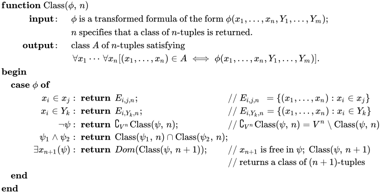
再帰的な コンピュータプログラムは、 与えられた式からクラスを構築する過程を簡潔に表現します。このプログラムの定義は、クラス存在定理の証明に依存しません。ただし、プログラムによって構築されたクラスが与えられた式を満たし、公理を用いて構築されていることを証明するには、その証明が必要です。このプログラムは、Pascal スタイルのcase 文 を用いた擬似コード で記述されています。[ i ] f u n c t 私 o n クラス ( ϕ 、 n ) 私 n p u t : ϕ は、次の形式の変換された式です。 ϕ ( x 1 、 … 、 x n 、 Y 1 、 … 、 Y m ) ; n クラスの n -タプルが返されます。 o u t p u t : クラス A の n -タプルが満たす ∀ x 1 ⋯ ∀ x n [ ( x 1 、 … 、 x n ) ∈ A ⟺ ϕ ( x 1 、 … 、 x n 、 Y 1 、 … 、 Y m ) ] 。 b e g 私 n c 1 s e ϕ o f x 私 ∈ x j : r e t u r n E 私 、 j 、 n ; // E 私 、 j 、 n = { ( x 1 、 … 、 x n ) : x 私 ∈ x j } x 私 ∈ Y k : r e t u r n E 私 、 Y k 、 n ; // E 私 、 Y k 、 n = { ( x 1 、 … 、 x n ) : x 私 ∈ Y k } ¬ ψ : r e t u r n ∁ V n クラス ( ψ 、 n ) ; // ∁ V n クラス ( ψ 、 n ) = V n ∖ クラス ( ψ 、 n ) ψ 1 ∧ ψ 2 : r e t u r n クラス ( ψ 1 、 n ) ∩ クラス ( ψ 2 、 n ) ; ∃ x n + 1 ( ψ ) : r e t u r n D o m ( クラス ( ψ 、 n + 1 ) ) ; // x n + 1 無料です ψ ; クラス ( ψ 、 n + 1 ) // のクラスを返します ( n + 1 ) -タプル e n d e n d {\displaystyle {\begin{array}{l}\mathbf {function} \;{\text{Class}}(\phi ,\,n)\\\quad {\begin{array}{rl}\mathbf {input} \!:\;\,&\phi {\text{ is a transformed formula of the form }}\phi (x_{1},\ldots ,x_{n},Y_{1},\ldots ,Y_{m});\\&n{\text{ specifies that a class of }}n{\text{-tuples is returned.}}\\\;\;\;\;\mathbf {output} \!:\;\,&{\text{class }}A{\text{ of }}n{\text{-tuples satisfying }}\\&\,\forall x_{1}\cdots \,\forall x_{n}[(x_{1},\ldots ,x_{n})\in A\iff \phi (x_{1},\ldots ,x_{n},Y_{1},\ldots ,Y_{m})].\end{array}}\\\mathbf {begin} \\\quad \mathbf {case} \;\phi \;\mathbf {of} \\\qquad {\begin{alignedat}{2}x_{i}\in x_{j}:\;\;&\mathbf {return} \;\,E_{i,j,n};&&{\text{// }}E_{i,j,n}\;\,=\{(x_{1},\dots ,x_{n}):x_{i}\in x_{j}\}\\x_{i}\in Y_{k}:\;\;&\mathbf {return} \;\,E_{i,Y_{k},n};&&{\text{// }}E_{i,Y_{k},n}=\{(x_{1},\dots ,x_{n}):x_{i}\in Y_{k}\}\\\neg \psi :\;\;&\mathbf {return} \;\,\complement _{V^{n}}{\text{Class}}(\psi ,\,n);&&{\text{// }}\complement _{V^{n}}{\text{Class}}(\psi ,\,n)=V^{n}\setminus {\text{Class}}(\psi ,\,n)\\\psi _{1}\land \psi _{2}:\;\;&\mathbf {return} \;\,{\text{Class}}(\psi _{1},\,n)\cap {\text{Class}}(\psi _{2},\,n);&&\\\;\;\;\;\,\exists x_{n+1}(\psi ):\;\;&\mathbf {return} \;\,Dom({\text{Class}}(\psi ,\,n+1));&&{\text{// }}x_{n+1}{\text{ は }}\psi で自由です ;{\text{ Class}}(\psi ,\,n+1)\\&\ &&{\text{// }}(n+1){\text{-タプル}}のクラスを返します\end{alignedat}}\\\quad \mathbf {end} \\\mathbf {end} \end{array}}}
ϕ {\displaystyle \phi } 例2 の式とする。関数呼び出しA = C l 1 s s ( ϕ 、 1 ) {\displaystyle A=Class(\phi ,1)} A 、 {\displaystyle A,} ϕ 。 {\displaystyle \phi .} A {\displaystyle A} ϕ 。 {\displaystyle \phi .}
ϕ = ∃ x 2 ( x 2 ∈ x 1 ∧ ¬ ∃ x 3 ( x 3 ∈ x 2 ) ) ∧ ∃ x 2 ( x 2 ∈ x 1 ∧ ∃ x 3 ( x 3 ∈ x 2 ∧ ¬ ∃ x 4 ( x 4 ∈ x 3 ) ) ) A = D o m ( E 2 、 1 、 2 ∩ ∁ V 2 D o m ( E 3 、 2 、 3 ) ) ∩ D o m ( E 2 、 1 、 2 ∩ D o m ( E 3 、 2 、 3 ∩ ∁ V 3 D o m ( E 4 、 3 、 4 ) ) ) {\displaystyle {\begin{alignedat}{2}&\phi \;&&=\;\;\exists x_{2}\,(x_{2}\!\in \!x_{1}\land \;\;\neg \;\;\;\;\exists x_{3}\;(x_{3}\!\in \!x_{2}))\,\land \;\;\,\exists x_{2}\,(x_{2}\!\in \!x_{1}\land \;\;\,\exists x_{3}\,(x_{3}\!\in \!x_{2}\,\land \;\;\neg \;\;\;\;\exists x_{4}\;(x_{4}\!\in \!x_{3})))\\&A\;&&=Dom\,(\;E_{2,1,2}\;\cap \;\complement _{V^{2}}\,Dom\,(\;E_{3,2,3}\;))\,\cap \,Dom\,(\;E_{2,1,2}\;\cap \,Dom\,(\;\,E_{3,2,3}\;\cap \;\complement _{V^{3}}\,Dom\,(\;E_{4,3,4}\;)))\end{alignedat}}}
クラス存在定理の拡張 ゲーデルはクラス存在定理を数式に拡張した。ϕ {\displaystyle \phi } クラス間の関係 を含む(例:Y 1 ⊆ Y 2 {\displaystyle Y_{1}\subseteq Y_{2}} 単項関係 M ( Y 1 ) {\displaystyle M(Y_{1})} O r d {\displaystyle Ord} 操作 (例:( x 1 、 x 2 ) {\displaystyle (x_{1},x_{2})} x 1 ∩ Y 1 {\displaystyle x_{1}\cap Y_{1}} [ ] 。 ϕ {\displaystyle \phi } クラス存在定理の仮説を 満たす等価な式に変換することができる。
以下の定義は、数式が関係、特殊クラス、および演算をどのように定義するかを示しています。
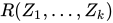
関係R {\displaystyle R} R ( Z 1 、 … 、 Z k ) ⟺ ψ R ( Z 1 、 … 、 Z k ) 。 {\displaystyle R(Z_{1},\dots ,Z_{k})\iff \psi _{R}(Z_{1},\dots ,Z_{k}).} 特別なクラスC {\displaystyle C} u ∈ C ⟺ ψ C ( u ) 。 {\displaystyle u\in C\iff \psi _{C}(u).} 手術P {\displaystyle P} u ∈ P ( Z 1 、 … 、 Z k ) ⟺ ψ P ( u 、 Z 1 、 … 、 Z k ) 。 {\displaystyle u\in P(Z_{1},\dots ,Z_{k})\iff \psi _{P}(u,Z_{1},\dots ,Z_{k}).} 用語は
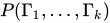
変数と特殊クラスは用語です。 もしP {\displaystyle P} k {\displaystyle k} Γ 1 、 … 、 Γ k {\displaystyle \Gamma _{1},\dots ,\Gamma _{k}} P ( Γ 1 、 … 、 Γ k ) {\displaystyle P(\Gamma _{1},\dots ,\Gamma _{k})} 以下の変換ルールは、関係、特殊クラス、および演算を削除します。ルール 2b、3b、または 4 がサブ式に適用されるたびに、私 {\displaystyle i} z 私 {\displaystyle z_{i}} Γ 1 、 … 、 Γ k 、 Γ 、 {\displaystyle \,\Gamma _{1},\dots ,\Gamma _{k},\Gamma ,} Δ {\displaystyle \Delta }
関係R ( Z 1 、 … 、 Z k ) {\displaystyle R(Z_{1},\dots ,Z_{k})} ψ R ( Z 1 、 … 、 Z k ) 。 {\displaystyle \psi _{R}(Z_{1},\dots ,Z_{k}).} させてψ C ( u ) {\displaystyle \psi _{C}(u)} C 。 {\displaystyle C.} Δ ∈ C {\displaystyle \Delta \in C} ψ C ( Δ ) 。 {\displaystyle \psi _{C}(\Delta ).} C ∈ Δ {\displaystyle C\in \Delta } ∃ z 私 [ z 私 = C ∧ z 私 ∈ Δ ] 。 {\displaystyle \exists z_{i}[z_{i}=C\land z_{i}\in \Delta ].} させてψ P ( u 、 Z 1 、 … 、 Z k ) {\displaystyle \psi _{P}(u,Z_{1},\dots ,Z_{k})} P ( Z 1 、 … 、 Z k ) 。 {\displaystyle P(Z_{1},\dots ,Z_{k}).} Δ ∈ P ( Γ 1 、 … 、 Γ k ) {\displaystyle \Delta \in P(\Gamma _{1},\dots ,\Gamma _{k})} ψ P ( Δ 、 Γ 1 、 … 、 Γ k ) 。 {\displaystyle \psi _{P}(\Delta ,\Gamma _{1},\dots ,\Gamma _{k}).} P ( Γ 1 、 … 、 Γ k ) ∈ Δ {\displaystyle P(\Gamma _{1},\dots ,\Gamma _{k})\in \Delta } ∃ z 私 [ z 私 = P ( Γ 1 、 … 、 Γ k ) ∧ z 私 ∈ Δ ] 。 {\displaystyle \exists z_{i}[z_{i}=P(\Gamma _{1},\dots ,\Gamma _{k})\land z_{i}\in \Delta ].} 外延性は変換するために用いられるΔ = Γ {\displaystyle \Delta =\Gamma } ∀ z 私 ( z 私 ∈ Δ ⟺ z 私 ∈ Γ ) 。 {\displaystyle \forall z_{i}(z_{i}\in \Delta \iff z_{i}\in \Gamma ).} クラス存在定理(拡張版 )— ϕ ( x 1 、 … 、 x n 、 Y 1 、 … 、 Y m ) {\displaystyle \phi (x_{1},\dots ,x_{n},Y_{1},\dots ,Y_{m})} x 1 、 … 、 x n 、 Y 1 、 … 、 Y m {\displaystyle x_{1},\dots ,x_{n},Y_{1},\dots ,Y_{m}} Y 1 、 … 、 Y m 、 {\displaystyle Y_{1},\dots ,Y_{m},} A {\displaystyle A} n {\displaystyle n} ∀ x 1 ⋯ ∀ x n [ ( x 1 、 … 、 x n ) ∈ A ⟺ ϕ ( x 1 、 … 、 x n 、 Y 1 、 … 、 Y m ) ] 。 {\displaystyle \forall x_{1}\cdots \,\forall x_{n}[(x_{1},\dots ,x_{n})\in A\iff \phi (x_{1},\dots ,x_{n},Y_{1},\dots ,Y_{m})].} [ j ]
証拠 変換ルールを適用してϕ {\displaystyle \phi } Y 1 、 … 、 Y m 、 {\displaystyle Y_{1},\dots ,Y_{m},} A {\displaystyle A} n {\displaystyle n} ∀ x 1 ⋯ ∀ x n [ ( x 1 、 … 、 x n ) ∈ A ⟺ ϕ ( x 1 、 … 、 x n 、 Y 1 、 … 、 Y m ) ] 。 {\displaystyle \forall x_{1}\cdots \,\forall x_{n}[(x_{1},\dots ,x_{n})\in A\iff \phi (x_{1},\dots ,x_{n},Y_{1},\dots ,Y_{m})].}
公理を設定する クラス存在定理の証明に必要なペアリング公理と正則性公理は既に述べた。NBGには他に4つの集合公理が含まれている。これらの公理のうち3つは、集合に適用されるクラス演算に関するものである。
意味。 F {\displaystyle F} 関数 である場合F ⊆ V 2 ∧ ∀ x ∀ y ∀ z [ ( x 、 y ) ∈ F ∧ ( x 、 z ) ∈ F ⟹ y = z ] 。 {\displaystyle F\subseteq V^{2}\land \forall x\,\forall y\,\forall z\,[(x,y)\in F\,\land \,(x,z)\in F\implies y=z].}
集合論では、関数の定義において、関数の定義域や終域を指定する必要はありません(「関数(集合論) 」を参照)。NBGの関数の定義は、ZFCの定義を順序対の集合から順序対のクラスへと一般化したものです。
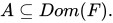
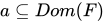
ZFCの像 、和集合 、冪集合 の集合演算の定義は、クラス演算にも一般化される。クラスの像A {\displaystyle A} F {\displaystyle F} F [ A ] = { y : ∃ x ( x ∈ A ∧ ( x 、 y ) ∈ F ) } 。 {\displaystyle F[A]=\{y:\exists x(x\in A\,\land \,(x,y)\in F)\}.} A ⊆ D o m ( F ) 。 {\displaystyle A\subseteq Dom(F).} A {\displaystyle A} ∪ A = { x : ∃ y ( x ∈ y ∧ y ∈ A ) } 。 {\displaystyle \cup A=\{x:\exists y(x\in y\,\,\land \,y\in A)\}.} A {\displaystyle A} P ( A ) = { x : x ⊆ A } 。 {\displaystyle {\mathcal {P}}(A)=\{x:x\subseteq A\}.} 和集合 、冪集合 の公理は、これらの操作を集合に適用すると集合が生成されることを意味する。[ 34 ]
置換公理 。F {\displaystyle F} 1 {\displaystyle a} F [ 1 ] {\displaystyle F[a]} イメージ 1 {\displaystyle a} F {\displaystyle F} ∀ F ∀ 1 [ F 関数です ⟹ ∃ b ∀ y ( y ∈ b ⟺ ∃ x ( x ∈ 1 ∧ ( x 、 y ) ∈ F ) ) ] 。 {\displaystyle \forall F\,\forall a\,[F{\text{ is a function}}\implies \exists b\,\forall y\,(y\in b\iff \exists x(x\in a\,\land \,(x,y)\in F))].}
要件を満たしていないA ⊆ D o m ( F ) {\displaystyle A\subseteq Dom(F)} F [ A ] {\displaystyle F[A]}
集合の公理。 1 {\displaystyle a} ∪ 1 。 {\displaystyle \cup a.} ∀ 1 ∃ b ∀ x [ ∃ y ( x ∈ y ∧ y ∈ 1 ) ⟹ x ∈ b ] 。 {\displaystyle \forall a\,\exists b\,\forall x\,[\,\exists y(x\in y\,\,\land \,y\in a)\implies x\in b\,].}
集合の公理。 1 {\displaystyle a} P ( 1 ) 。 {\displaystyle {\mathcal {P}}(a).}
∀ 1 ∃ b ∀ x ( x ⊆ 1 ⟹ x ∈ b ) 。 {\displaystyle \forall a\,\exists b\,\forall x\,(x\subseteq a\implies x\in b).} [ k ] 無限公理。 空でない集合が存在する。1 {\displaystyle a} x {\displaystyle x} 1 {\displaystyle a} y {\displaystyle y} 1 {\displaystyle a} x {\displaystyle x} y {\displaystyle y} ∃ 1 [ ∃ u ( u ∈ 1 ) ∧ ∀ x ( x ∈ 1 ⟹ ∃ y ( y ∈ 1 ∧ x ⊂ y ) ) ] 。 {\displaystyle \exists a\,[\exists u(u\in a)\,\land \,\forall x(x\in a\implies \exists y(y\in a\,\land \,x\subset y))].}
無限公理と置換公理は空集合 の存在を証明する。クラス存在公理の議論 では、空クラスの存在が証明される。∅ {\displaystyle \emptyset } ∅ {\displaystyle \emptyset } F = ∅ {\displaystyle F=\emptyset } 1 {\displaystyle a} 1 {\displaystyle a} F {\displaystyle F} ∅ {\displaystyle \emptyset }
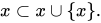
NBGの無限公理はZFCの無限公理 によって暗示される。∃ 1 [ ∅ ∈ 1 ∧ ∀ x ( x ∈ 1 ⟹ x ∪ { x } ∈ 1 ) ] 。 {\displaystyle \,\exists a\,[\emptyset \in a\,\land \,\forall x(x\in a\implies x\cup \{x\}\in a)].\,} 連言は、 ∅ ∈ 1 {\displaystyle \emptyset \in a} ∀ x ( x ∈ 1 ⟹ x ∪ { x } ∈ 1 ) {\displaystyle \forall x(x\in a\implies x\cup \{x\}\in a)} x ⊂ x ∪ { x } 。 {\displaystyle x\subset x\cup \{x\}.} 弱い無限公理を 参照)。[ l ]






![{\displaystyle \forall x_{1}\cdots \,\forall x_{n}[(x_{1},\ldots ,x_{n})\in A\iff \phi (x_{1},\ldots ,x_{n})].}](https://wikimedia.org/api/rest_v1/media/math/render/svg/5a4bbd44672be9c44edc7e27e7f4d0fe21ff8874)






![{\displaystyle \forall A\,\forall B\,[\forall x(x\in A\iff x\in B)\implies A=B]}](https://wikimedia.org/api/rest_v1/media/math/render/svg/241eef7d867be06ecf35bcb9a4dce9da32626e88)


![{\displaystyle \forall x\,\forall y\,\exists p\,\forall z\,[z\in p\iff (z=x\,\lor \,z=y)]}](https://wikimedia.org/api/rest_v1/media/math/render/svg/43f8175b900322da6f061d58dd643352a0a5e50e)





![{\displaystyle \exists E\,\forall x\,\forall y\,[(x,y)\in E\iff x\in y]\!}](https://wikimedia.org/api/rest_v1/media/math/render/svg/75b6597b3f8f7f040da8f637d9a5307597f3a1f1)

![{\displaystyle \forall A\,\forall B\,\exists C\,\forall x\,[x\in C\iff (x\in A\,\land \,x\in B)]}](https://wikimedia.org/api/rest_v1/media/math/render/svg/197b276873b716c1a83d1d94af367862900da1ea)
![{\displaystyle \forall A\,\exists B\,\forall x\,[x\in B\iff \neg (x\in A)]}](https://wikimedia.org/api/rest_v1/media/math/render/svg/9450bca22cfc5d874901ba0d44b3539147e574e0)
![{\displaystyle \forall A\,\exists B\,\forall x\,[x\in B\iff \exists y((x,y)\in A)]}](https://wikimedia.org/api/rest_v1/media/math/render/svg/f22c660ba2347b6dd6014ac3a26e833bc0caedb9)


![{\displaystyle \forall A\,\exists B\,\forall u\,[u\in B\iff \exists x\,\exists y\,(u=(x,y)\land x\in A)]}](https://wikimedia.org/api/rest_v1/media/math/render/svg/c2f45de53d4e2ee4c42622d59563b91a4a5dd8e7)

![{\displaystyle \forall A\,\exists B\,\forall x\,\forall y\,\forall z\,[(x,y,z)\in B\iff (y,z,x)\in A]}](https://wikimedia.org/api/rest_v1/media/math/render/svg/ecb3d73e80a870caf94253aa8afab0a8e885af66)
![{\displaystyle \forall A\,\exists B\,\forall x\,\forall y\,\forall z\,[(x,y,z)\in B\iff (x,z,y)\in A]}](https://wikimedia.org/api/rest_v1/media/math/render/svg/1ceb9de8295c9ca52de2c8965cdc8e4dd1f72913)






![{\displaystyle \forall A\,\exists B_{1}\,\forall x\,\forall y\,\forall z\,[(z,x,y)\in B_{1}\iff (x,y)\in A]}](https://wikimedia.org/api/rest_v1/media/math/render/svg/0551e12143886cea9a751fced7944423cc218627)
![{\displaystyle \forall A\,\exists B_{2}\,\forall x\,\forall y\,\forall z\,[(x,z,y)\in B_{2}\iff (x,y)\in A]}](https://wikimedia.org/api/rest_v1/media/math/render/svg/6b6993cde8ec20c99d868ca5fd8a0b1adbda0bf4)
![{\displaystyle \forall A\,\exists B_{3}\,\forall x\,\forall y\,\forall z\,[(x,y,z)\in B_{3}\iff (x,y)\in A]}](https://wikimedia.org/api/rest_v1/media/math/render/svg/2e4d1d6722e06510dfc69706454d60d3f63c3055)
![{\displaystyle \forall A\,\exists B_{4}\,\forall x\,\forall y\,\forall z\,[(y,x)\in B_{4}\iff (x,y)\in A]}](https://wikimedia.org/api/rest_v1/media/math/render/svg/d0be69b28701384ef168ff9bfffd671d7690ad35)


![{\displaystyle \forall a\,[a\neq \emptyset \implies \exists u(u\in a\land u\cap a=\emptyset )].}](https://wikimedia.org/api/rest_v1/media/math/render/svg/be47d555db4994e987a277a26740c151d0f0c3a6)






![{\displaystyle \forall x_{1}\cdots \,\forall x_{n}[(x_{1},\dots ,x_{n})\in A\iff \phi (x_{1},\dots ,x_{n},Y_{1},\dots ,Y_{m})].}](https://wikimedia.org/api/rest_v1/media/math/render/svg/85ed8313491a2c7b4011ab9a536a751e08a96620)









![\displaystyle \exists t[(x_{1},t)\in F\,\land \,(t,x_{2})\in G].}](https://wikimedia.org/api/rest_v1/media/math/render/svg/bcf0a1c1a26717a495dc5ef5f1e35b285430cceb)





























![{\displaystyle \forall x_{1}\cdots \,\forall x_{n}[(x_{1},\ldots ,x_{n})\in A\iff \phi (x_{1},\ldots ,x_{n},Y_{1},\ldots ,Y_{m})].}](https://wikimedia.org/api/rest_v1/media/math/render/svg/efbe3e28e60323770b9db02c02a02d6aaadd0a3c)



















![{\displaystyle \forall u\,[u\in \complement (A)\iff \neg (u\in A)].}](https://wikimedia.org/api/rest_v1/media/math/render/svg/41c9fb3cef985276c75ebb99d6b614aa77a1e5e3)


![{\displaystyle {\begin{alignedat}{2}\quad &(x_{1},\ldots ,x_{n})\in \complement _{V^{n}}(A)&&\iff \neg [(x_{1},\ldots ,x_{n})\in A]\\&&&\iff \neg \psi (x_{1},\ldots ,x_{n},{\vec {Y}})\\&&&\iff \phi (x_{1},\ldots ,x_{n},{\vec {Y}}).\end{alignedat}}}](https://wikimedia.org/api/rest_v1/media/math/render/svg/fce2ccab49fecd78319fbb123b977bf4cdb57f9d)











![{\displaystyle {\begin{alignedat}{2}\quad &(x_{1},\ldots ,x_{n})\in Dom(A)&&\iff \exists x_{n+1}[((x_{1},\ldots ,x_{n}),x_{n+1})\in A]\\&&&\iff \exists x_{n+1}[(x_{1},\ldots ,x_{n},x_{n+1})\in A]\\&&&\iff \exists x_{n+1}\,\psi (x_{1},\ldots ,x_{n},x_{n+1},{\vec {Y}})\\&&&\iff \phi (x_{1},\ldots ,x_{n},{\vec {Y}}).\end{alignedat}}}](https://wikimedia.org/api/rest_v1/media/math/render/svg/d1814606d89e7d61c7a3dc3fb82b98b724275c16)













![{\displaystyle \exists z_{i}[z_{i}=C\land z_{i}\in \Delta ].}](https://wikimedia.org/api/rest_v1/media/math/render/svg/cd71799ec11db6723266d1bfb4a8dbb15314fe16)





![{\displaystyle \exists z_{i}[z_{i}=P(\Gamma _{1},\dots ,\Gamma _{k})\land z_{i}\in \Delta ].}](https://wikimedia.org/api/rest_v1/media/math/render/svg/c7f187eaecdc751d265379015ab3870dc6734f0a)


![{\displaystyle F\subseteq V^{2}\land \forall x\,\forall y\,\forall z\,[(x,y)\in F\,\land \,(x,z)\in F\implies y=z].}](https://wikimedia.org/api/rest_v1/media/math/render/svg/39e46fe8c2c518a6c07dfb3747ad4dc24f3802f4)
![{\displaystyle F[A]=\{y:\exists x(x\in A\,\land \,(x,y)\in F)\}.}](https://wikimedia.org/api/rest_v1/media/math/render/svg/3adcf4bbc0fba47d1b068d2863ba2840440d3fde)


![{\displaystyle F[a]}](https://wikimedia.org/api/rest_v1/media/math/render/svg/7c8e90bfcbe7e0bb619096b7c0d91b12cb7c20f4)
![{\displaystyle \forall F\,\forall a\,[F{\text{は関数である}}\implies \exists b\,\forall y\,(y\in b\iff \exists x(x\in a\,\land \,(x,y)\in F))].}](https://wikimedia.org/api/rest_v1/media/math/render/svg/7d5be626156ac915fe374ffe54da1a3a407186fa)

![{\displaystyle F[A]}](https://wikimedia.org/api/rest_v1/media/math/render/svg/667bb1fca53d019ead801661a56c8afeeb4bef8c)






![{\displaystyle \forall a\,\exists b\,\forall x\,[\,\exists y(x\in y\,\,\land \,y\in a)\implies x\in b\,].}](https://wikimedia.org/api/rest_v1/media/math/render/svg/bcd5515f243541353f13ac8782936e9b36dfa8f0)




![{\displaystyle \exists a\,[\exists u(u\in a)\,\land \,\forall x(x\in a\implies \exists y(y\in a\,\land \,x\subset y))].}](https://wikimedia.org/api/rest_v1/media/math/render/svg/c404faf2bfdd821d5ebbf7a3957d6c2eeaeafaa1)

![{\displaystyle \,\exists a\,[\emptyset \in a\,\land \,\forall x(x\in a\implies x\cup \{x\}\in a)].\,}](https://wikimedia.org/api/rest_v1/media/math/render/svg/5a33dea5048bde96a5aa4be13cfcacc9fc38d0e6)




![{\displaystyle \exists G\,[G{\text{は関数である}}\,\land \forall x(x\neq \emptyset \implies \exists y(y\in x\land (x,y)\in G))].}](https://wikimedia.org/api/rest_v1/media/math/render/svg/fb1b7fd53af984df9ed30029df16a95bf72f35ae)





![{\displaystyle E=\{x\in V_{\kappa }:(V_{\kappa },\in )\models \exists u\ \exists v[x=(u,v)\land u\in v]\}.}](https://wikimedia.org/api/rest_v1/media/math/render/svg/3adaeacce71ec9b637fbe8b57b3b2d277259f962)
![{\displaystyle E=\{x\in L_{\kappa }:(L_{\kappa },\in )\models \exists u\ \exists v[x=(u,v)\land u\in v]\}.}](https://wikimedia.org/api/rest_v1/media/math/render/svg/64231382a0b2b3ae97752075dbbdc0dc52bf498e)




![{\displaystyle \exists x[\exists C(x\in C)\land \phi (x)].}](https://wikimedia.org/api/rest_v1/media/math/render/svg/07e54b528d4fbd7d3473d7d35c3789b8930bf6d0)
![{\displaystyle \exists x[x\in V\land \phi (x)].}](https://wikimedia.org/api/rest_v1/media/math/render/svg/77dd05b7deeb3a51bbb181a013bc40680ce0790f)
![{\displaystyle \exists x_{n+1}[x_{n+1}\land \dots ]}](https://wikimedia.org/api/rest_v1/media/math/render/svg/fbcb706d5afa593a4200e67fea72609f8f553034)
![{\displaystyle \exists x_{n+1}[x_{n+1}\in V\land \dots ],}](https://wikimedia.org/api/rest_v1/media/math/render/svg/8e28329f94ea425552e058ef34bd83c47100f8b0)
![{\displaystyle A\times B=\{x:\exists y\exists z[x=(y,z)\land y\in A\land z\in B]\},}](https://wikimedia.org/api/rest_v1/media/math/render/svg/908967fd22005a7f84cadb4bedc1d89b3af6f3e2)







![{\displaystyle \alpha (x)={\text{least}}\,\{\alpha :\exists y[(x,y)\in R\cap V_{\alpha }]\}}](https://wikimedia.org/api/rest_v1/media/math/render/svg/a52e0a6ba57a87c7cbe3869edcc8b0a94c4b0bc0)





