ベクトル空間からそれ自身へのべき等線形変換
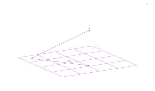
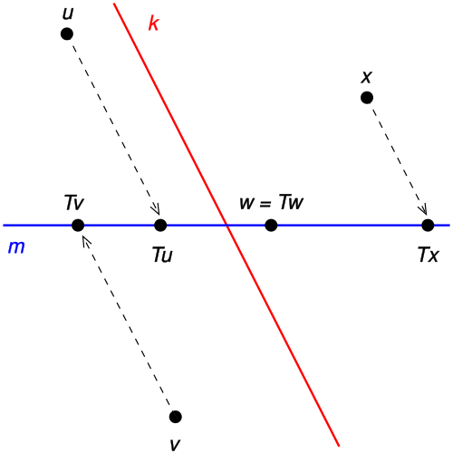
変換 P は 線分 m へ の 直交投影です 。 線型代数 と 関数解析 において 、 射影とは ベクトル空間 から それ自身への 線型変換( 自己準同型 )であり 、 となる 。つまり、を 任意のベクトルに 2 回適用すると、 を 1 回適用した場合と同じ結果が得られる(つまり、 はべき等性 となる )。その 像は 変化しない。 [1]この「射影」の定義は、 グラフィカル射影 の考え方を形式化し一般化するもので ある。また、射影が幾何学的オブジェクトに与える影響は、 オブジェクト内の
点に与える影響を調べることによっても検討できる。
ポ
{\displaystyle P}
ポ ∘ ポ = ポ
{\displaystyle P\circ P=P}
ポ
{\displaystyle P}
ポ
{\displaystyle P}
定義 ベクトル空間への 射影 は 、 となるような 線形演算子です 。
五
{\displaystyle V}
ポ : 五 → 五
{\displaystyle P\colon V\to V}
ポ
2
= ポ
{\displaystyle P^{2}=P}
が内積を 持ち 、 が 完備な 場合 、つまり が ヒルベルト空間 である場合、 直交性 の概念 を使用できます。 ヒルベルト空間への射影は、 すべての に対して を満たす場合、 直交射影 と呼ばれます 。 直交していないヒルベルト空間への射影は 斜射影 と呼ばれます。
五
{\displaystyle V}
五
{\displaystyle V}
ポ
{\displaystyle P}
五
{\displaystyle V}
⟨ ポ
x
、
ええ
⟩ = ⟨
x
、 ポ
ええ
⟩
{\displaystyle \langle P\mathbf {x} ,\mathbf {y} \rangle =\langle \mathbf {x} ,P\mathbf {y} \rangle }
x
、
ええ
∈ 五
{\displaystyle \mathbf {x} ,\mathbf {y} \in V}
投影行列 正方行列は、 その 平方に等しい場合、すなわち の場合、 射影行列 と呼ばれます 。 [2] : p. 38
ポ
{\displaystyle P}
ポ
2
= ポ
{\displaystyle P^{2}=P}
正方行列は、 実行 行列 の ときは 直交射影行列 と呼ばれ 、 複素 行列 のときはそれぞれ となる。ここで は の 転置 を表し 、は の 随伴転置または エルミート転置 を表す。 [2] : p. 223
ポ
{\displaystyle P}
ポ
2
= ポ =
ポ
T
{\displaystyle P^{2}=P=P^{\mathrm {T} }}
P
2
=
P
=
P
∗
{\displaystyle P^{2}=P=P^{*}}
P
T
{\displaystyle P^{\mathrm {T} }}
P
{\displaystyle P}
P
∗
{\displaystyle P^{*}}
P
{\displaystyle P}
直交射影行列ではない射影行列を 斜射射影行列 と呼びます。 投影行列の固有値は 0 または 1 でなければなりませ
ん 。
例
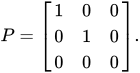
正射影 例えば、 3次元空間の点 を点に写像する関数は、 xy 平面への直交投影である 。この関数は、行列で表される。
(
x
,
y
,
z
)
{\displaystyle (x,y,z)}
R
3
{\displaystyle \mathbb {R} ^{3}}
(
x
,
y
,
0
)
{\displaystyle (x,y,0)}
P
=
[
1
0
0
0
1
0
0
0
0
]
.
{\displaystyle P={\begin{bmatrix}1&0&0\\0&1&0\\0&0&0\end{bmatrix}}.}
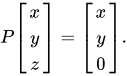
この行列の任意のベクトル に対する作用 は
P
[
x
y
z
]
=
[
x
y
0
]
.
{\displaystyle P{\begin{bmatrix}x\\y\\z\end{bmatrix}}={\begin{bmatrix}x\\y\\0\end{bmatrix}}.}
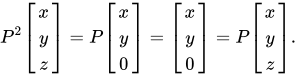
が実際に射影である ことを確認するために 、すなわち を計算する。
P
{\displaystyle P}
P
=
P
2
{\displaystyle P=P^{2}}
P
2
[
x
y
z
]
=
P
[
x
y
0
]
=
[
x
y
0
]
=
P
[
x
y
z
]
.
{\displaystyle P^{2}{\begin{bmatrix}x\\y\\z\end{bmatrix}}=P{\begin{bmatrix}x\\y\\0\end{bmatrix}}={\begin{bmatrix}x\\y\\0\end{bmatrix}}=P{\begin{bmatrix}x\\y\\z\end{bmatrix}}.}
これを観察すると 、投影が正射影であることがわかります。
P
T
=
P
{\displaystyle P^{\mathrm {T} }=P}
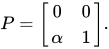
斜投影 非直交(斜交)投影の簡単な例は次の通りです。
P
=
[
0
0
α
1
]
.
{\displaystyle P={\begin{bmatrix}0&0\\\alpha &1\end{bmatrix}}.}
行列の乗算 により 、
が 実際に投影である
ことを示すことがわかります。
P
2
=
[
0
0
α
1
]
[
0
0
α
1
]
=
[
0
0
α
1
]
=
P
.
{\displaystyle P^{2}={\begin{bmatrix}0&0\\\alpha &1\end{bmatrix}}{\begin{bmatrix}0&0\\\alpha &1\end{bmatrix}}={\begin{bmatrix}0&0\\\alpha &1\end{bmatrix}}=P.}
P
{\displaystyle P}
投影 が直交する のは、 その場合のみである。
P
{\displaystyle P}
α
=
0
{\displaystyle \alpha =0}
P
T
=
P
.
{\displaystyle P^{\mathrm {T} }=P.}
特性と分類 変換 T は、 kに沿った m への 射影です。 T の値域は m で 、核は k です。
冪等性 定義により、射影は べき等性 (つまり) があります 。
P
{\displaystyle P}
P
2
=
P
{\displaystyle P^{2}=P}
地図を開く すべての投影は 開写像であり、 領域 内の 各 開集合を 画像 の 部分空間位相 内の開集合に写像することを意味します 。 [ 要出典 ] つまり、任意のベクトル と を中心とする任意の球 (正の半径を持つ) に対して、 画像 に完全に含まれる を中心とする 球 (正の半径を持つ)が存在します 。
x
{\displaystyle \mathbf {x} }
B
x
{\displaystyle B_{\mathbf {x} }}
x
{\displaystyle \mathbf {x} }
B
P
x
{\displaystyle B_{P\mathbf {x} }}
P
x
{\displaystyle P\mathbf {x} }
P
(
B
x
)
{\displaystyle P(B_{\mathbf {x} })}
イメージとカーネルの相補性 を有限次元ベクトル空間とし、 を への射影とします 。 部分空間 と がそれぞれ の 像 と 核 で あるとします 。すると には 次の特性があります。
W
{\displaystyle W}
P
{\displaystyle P}
W
{\displaystyle W}
U
{\displaystyle U}
V
{\displaystyle V}
P
{\displaystyle P}
P
{\displaystyle P}
P
{\displaystyle P}
は上の 恒等演算子 です :
I
{\displaystyle I}
U
{\displaystyle U}
∀
x
∈
U
:
P
x
=
x
.
{\displaystyle \forall \mathbf {x} \in U:P\mathbf {x} =\mathbf {x} .}
直和 が 成り立ちます 。すべてのベクトルは および で 一意 に分解でき 、ここで
W
=
U
⊕
V
{\displaystyle W=U\oplus V}
x
∈
W
{\displaystyle \mathbf {x} \in W}
x
=
u
+
v
{\displaystyle \mathbf {x} =\mathbf {u} +\mathbf {v} }
u
=
P
x
{\displaystyle \mathbf {u} =P\mathbf {x} }
v
=
x
−
P
x
=
(
I
−
P
)
x
{\displaystyle \mathbf {v} =\mathbf {x} -P\mathbf {x} =\left(I-P\right)\mathbf {x} }
u
∈
U
,
v
∈
V
.
{\displaystyle \mathbf {u} \in U,\mathbf {v} \in V.}
射影の像と核は 相補的 であり、 と も同様です。 の 像と核は の 核と像になり、その逆もまた同様であるため、 演算子も射影です。 は (核/像) への 射影であり 、 は へ の射影であると 言えます 。
P
{\displaystyle P}
Q
=
I
−
P
{\displaystyle Q=I-P}
Q
{\displaystyle Q}
P
{\displaystyle P}
Q
{\displaystyle Q}
P
{\displaystyle P}
V
{\displaystyle V}
U
{\displaystyle U}
Q
{\displaystyle Q}
U
{\displaystyle U}
V
{\displaystyle V}
スペクトラム 無限次元ベクトル空間では、 射影の スペクトル は に次のように
含まれます 。射影の 固有値
は 0 または 1 のみです。これは、直交射影 が常に 半正定値行列 であることを意味します。一般に、対応する 固有空間は (それぞれ) 射影の核と値域です。ベクトル空間の直和への分解は一意ではありません。したがって、部分空間 が与えられた場合 、値域 (または核) が である射影が多数存在する可能性があります 。
{
0
,
1
}
{\displaystyle \{0,1\}}
(
λ
I
−
P
)
−
1
=
1
λ
I
+
1
λ
(
λ
−
1
)
P
.
{\displaystyle (\lambda I-P)^{-1}={\frac {1}{\lambda }}I+{\frac {1}{\lambda (\lambda -1)}}P.}
P
{\displaystyle P}
V
{\displaystyle V}
V
{\displaystyle V}
射影が自明でない場合、それは 最小の多項式 を持ち、それは異なる線形因子に因数分解されるため、対 角化可能 です 。
x
2
−
x
=
x
(
x
−
1
)
{\displaystyle x^{2}-x=x(x-1)}
P
{\displaystyle P}
投影の製品 射影の積は、たとえ直交していても、一般に射影ではありません。2 つの射影が可換であれば、 その 積は射影になりますが、その 逆 は偽です。つまり、2 つの非可換射影の積は射影になることがあります。
2 つの直交射影が可換である場合、それらの積は直交射影です。2 つの直交射影の積が直交射影である場合、2 つの直交射影は可換です (より一般的には、2 つの自己随伴自己 準同型は 、それらの積が自己随伴である場合にのみ可換です)。
直交投影 ベクトル空間が 内積を 持ち 、完備( ヒルベルト空間)である場合、 直交性 の概念 を使用できます。 直交射影 とは、範囲 と核 が 直交部分空間 である射影です。したがって、 の任意のおよび に対して 、となります 。 これは同等です。
W
{\displaystyle W}
U
{\displaystyle U}
V
{\displaystyle V}
x
{\displaystyle \mathbf {x} }
y
{\displaystyle \mathbf {y} }
W
{\displaystyle W}
⟨
P
x
,
(
y
−
P
y
)
⟩
=
⟨
(
x
−
P
x
)
,
P
y
⟩
=
0
{\displaystyle \langle P\mathbf {x} ,(\mathbf {y} -P\mathbf {y} )\rangle =\langle (\mathbf {x} -P\mathbf {x} ),P\mathbf {y} \rangle =0}
⟨
x
,
P
y
⟩
=
⟨
P
x
,
P
y
⟩
=
⟨
P
x
,
y
⟩
.
{\displaystyle \langle \mathbf {x} ,P\mathbf {y} \rangle =\langle P\mathbf {x} ,P\mathbf {y} \rangle =\langle P\mathbf {x} ,\mathbf {y} \rangle .}
射影が直交する場合、かつその場合のみ、それが 自己随伴 である。 の自己随伴性と冪等性を利用すると 、 の任意の および に対して 、 、 、
が成り立ちます。
ここで は に関連付けられた内積です 。したがって、 および は 直交射影です。 [3] もう一方の方向、つまり が直交する場合、 は自己随伴であるという方向は、 および における
任意のに対して から へ
の含意から導かれます。 したがって です 。
P
{\displaystyle P}
x
{\displaystyle \mathbf {x} }
y
{\displaystyle \mathbf {y} }
W
{\displaystyle W}
P
x
∈
U
{\displaystyle P\mathbf {x} \in U}
y
−
P
y
∈
V
{\displaystyle \mathbf {y} -P\mathbf {y} \in V}
⟨
P
x
,
y
−
P
y
⟩
=
⟨
x
,
(
P
−
P
2
)
y
⟩
=
0
{\displaystyle \langle P\mathbf {x} ,\mathbf {y} -P\mathbf {y} \rangle =\langle \mathbf {x} ,\left(P-P^{2}\right)\mathbf {y} \rangle =0}
⟨
⋅
,
⋅
⟩
{\displaystyle \langle \cdot ,\cdot \rangle }
W
{\displaystyle W}
P
{\displaystyle P}
I
−
P
{\displaystyle I-P}
P
{\displaystyle P}
⟨
(
x
−
P
x
)
,
P
y
⟩
=
⟨
P
x
,
(
y
−
P
y
)
⟩
=
0
{\displaystyle \langle (\mathbf {x} -P\mathbf {x} ),P\mathbf {y} \rangle =\langle P\mathbf {x} ,(\mathbf {y} -P\mathbf {y} )\rangle =0}
⟨
x
,
P
y
⟩
=
⟨
P
x
,
P
y
⟩
=
⟨
P
x
,
y
⟩
=
⟨
x
,
P
∗
y
⟩
{\displaystyle \langle \mathbf {x} ,P\mathbf {y} \rangle =\langle P\mathbf {x} ,P\mathbf {y} \rangle =\langle P\mathbf {x} ,\mathbf {y} \rangle =\langle \mathbf {x} ,P^{*}\mathbf {y} \rangle }
x
{\displaystyle x}
y
{\displaystyle y}
W
{\displaystyle W}
P
=
P
∗
{\displaystyle P=P^{*}}
ヒルベルト射影定理 から、閉部分空間への直交射影の存在が分かります 。
プロパティと特殊なケース 直交射影は 有界演算子 です。これは、ベクトル空間の任意の に対して、 コーシー・シュワルツの不等式 により が成り立つためです 。
したがって 。
v
{\displaystyle \mathbf {v} }
‖
P
v
‖
2
=
⟨
P
v
,
P
v
⟩
=
⟨
P
v
,
v
⟩
≤
‖
P
v
‖
⋅
‖
v
‖
{\displaystyle \left\|P\mathbf {v} \right\|^{2}=\langle P\mathbf {v} ,P\mathbf {v} \rangle =\langle P\mathbf {v} ,\mathbf {v} \rangle \leq \left\|P\mathbf {v} \right\|\cdot \left\|\mathbf {v} \right\|}
‖
P
v
‖
≤
‖
v
‖
{\displaystyle \left\|P\mathbf {v} \right\|\leq \left\|\mathbf {v} \right\|}
有限次元の複素ベクトル空間または実ベクトル空間の場合、 の代わりに 標準の内積 を使用できます。
⟨
⋅
,
⋅
⟩
{\displaystyle \langle \cdot ,\cdot \rangle }
直交射影が直線上に投影されるときは、単純なケースになります。 が直線上の 単位ベクトル である場合 、射影は外積によって与えられます (
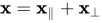
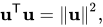
が 複素数値である場合、上式の転置はエルミート転置に置き換えられます)。 この演算子は u を 不変のままにし、 に直交するすべてのベクトルを消滅させ、それが確かに u を 含む直線上への直交射影であることを証明します 。 [4] これを確認する簡単な方法は、任意のベクトルを直線上の成分 (つまり、求める射影ベクトル) とそれに垂直な別の成分 の和として 考えることです。 射影を適用すると、平行ベクトルと垂直ベクトルの ドット積
の特性によって が得られます
。
u
{\displaystyle \mathbf {u} }
P
u
=
u
u
T
.
{\displaystyle P_{\mathbf {u} }=\mathbf {u} \mathbf {u} ^{\mathsf {T}}.}
u
{\displaystyle \mathbf {u} }
u
{\displaystyle \mathbf {u} }
x
{\displaystyle \mathbf {x} }
x
=
x
∥
+
x
⊥
{\displaystyle \mathbf {x} =\mathbf {x} _{\parallel }+\mathbf {x} _{\perp }}
P
u
x
=
u
u
T
x
∥
+
u
u
T
x
⊥
=
u
(
sgn
(
u
T
x
∥
)
‖
x
∥
‖
)
+
u
⋅
0
=
x
∥
{\displaystyle P_{\mathbf {u} }\mathbf {x} =\mathbf {u} \mathbf {u} ^{\mathsf {T}}\mathbf {x} _{\parallel }+\mathbf {u} \mathbf {u} ^{\mathsf {T}}\mathbf {x} _{\perp }=\mathbf {u} \left(\operatorname {sgn} \left(\mathbf {u} ^{\mathsf {T}}\mathbf {x} _{\parallel }\right)\left\|\mathbf {x} _{\parallel }\right\|\right)+\mathbf {u} \cdot \mathbf {0} =\mathbf {x} _{\parallel }}
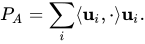
この式は、任意の次元 の部分空間への直交射影に一般化できる 。 整数 を仮定して、 部分空間 の 正規直交基底 を とし 、 列が である行列 、すなわち とすると 、射影は次のように表される: [5]
これは次のように書き直すことができる
:
u
1
,
…
,
u
k
{\displaystyle \mathbf {u} _{1},\ldots ,\mathbf {u} _{k}}
U
{\displaystyle U}
k
≥
1
{\displaystyle k\geq 1}
A
{\displaystyle A}
n
×
k
{\displaystyle n\times k}
u
1
,
…
,
u
k
{\displaystyle \mathbf {u} _{1},\ldots ,\mathbf {u} _{k}}
A
=
[
u
1
⋯
u
k
]
{\displaystyle A={\begin{bmatrix}\mathbf {u} _{1}&\cdots &\mathbf {u} _{k}\end{bmatrix}}}
P
A
=
A
A
T
{\displaystyle P_{A}=AA^{\mathsf {T}}}
P
A
=
∑
i
⟨
u
i
,
⋅
⟩
u
i
.
{\displaystyle P_{A}=\sum _{i}\langle \mathbf {u} _{i},\cdot \rangle \mathbf {u} _{i}.}
行列 は の 直交補行列 上で消える 部分等長行列 であり 、 は基になるベクトル空間に 埋め込まれる等長行列です。 したがって、 の値域は の 最終的な空間 です。が 上の恒等演算子である ことも明らかです 。
A
T
{\displaystyle A^{\mathsf {T}}}
U
{\displaystyle U}
A
{\displaystyle A}
U
{\displaystyle U}
P
A
{\displaystyle P_{A}}
A
{\displaystyle A}
A
A
T
{\displaystyle AA^{\mathsf {T}}}
U
{\displaystyle U}
正規直交性条件も省略できる。 が (必ずしも正規直交とは限らない) 基底 で が これらのベクトルを列として持つ行列である場合、射影は次のようになる: [6] [7]
u
1
,
…
,
u
k
{\displaystyle \mathbf {u} _{1},\ldots ,\mathbf {u} _{k}}
k
≥
1
{\displaystyle k\geq 1}
A
{\displaystyle A}
P
A
=
A
(
A
T
A
)
−
1
A
T
.
{\displaystyle P_{A}=A\left(A^{\mathsf {T}}A\right)^{-1}A^{\mathsf {T}}.}
行列は 依然として 基になるベクトル空間に埋め込まれますが、一般に等長行列ではなくなります。行列は、 ノルムを回復する「正規化係数」です。たとえば、 階数 -1 の演算子は 、 を で割った後、 によって張られる部分空間への 射影を得る 場合、射影ではありません 。
A
{\displaystyle A}
U
{\displaystyle U}
(
A
T
A
)
−
1
{\displaystyle \left(A^{\mathsf {T}}A\right)^{-1}}
u
u
T
{\displaystyle \mathbf {u} \mathbf {u} ^{\mathsf {T}}}
‖
u
‖
≠
1.
{\displaystyle \left\|\mathbf {u} \right\|\neq 1.}
u
T
u
=
‖
u
‖
2
,
{\displaystyle \mathbf {u} ^{\mathsf {T}}\mathbf {u} =\left\|\mathbf {u} \right\|^{2},}
u
(
u
T
u
)
−
1
u
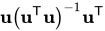
T
{\displaystyle \mathbf {u} \left(\mathbf {u} ^{\mathsf {T}}\mathbf {u} \right)^{-1}\mathbf {u} ^{\mathsf {T}}}
u
{\displaystyle u}
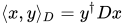
一般的な場合、内積を定義する任意の 正定値 行列 があり 、その射影は で与えられる 。すると、
D
{\displaystyle D}
⟨
x
,
y
⟩
D
=
y
†
D
x
{\displaystyle \langle x,y\rangle _{D}=y^{\dagger }Dx}
P
A
{\displaystyle P_{A}}
P
A
x
=
argmin
y
∈
range
(
A
)
‖
x
−
y
‖
D
2
{\textstyle P_{A}x=\operatorname {argmin} _{y\in \operatorname {range} (A)}\left\|x-y\right\|_{D}^{2}}
P
A
=
A
(
A
T
D
A
)
−
1
A
T
D
.
{\displaystyle P_{A}=A\left(A^{\mathsf {T}}DA\right)^{-1}A^{\mathsf {T}}D.}
射影の値域空間が フレーム によって生成される場合(つまり、生成元の数がその次元よりも大きい場合)、射影の式は次の形式になります。 ここで は ムーア・ペンローズ擬似逆行列 を表します 。これは、射影演算子を構築する多くの方法の 1 つにすぎません。
P
A
=
A
A
+
{\displaystyle P_{A}=AA^{+}}
A
+
{\displaystyle A^{+}}
が非特異行列であり、 (すなわち、が の ヌル空間 行列 である) 場合 、 [8] 以下が成り立ちます。
[
A
B
]
{\displaystyle {\begin{bmatrix}A&B\end{bmatrix}}}
A
T
B
=
0
{\displaystyle A^{\mathsf {T}}B=0}
B
{\displaystyle B}
A
{\displaystyle A}
I
=
[
A
B
]
[
A
B
]
−
1
[
A
T
B
T
]
−
1
[
A
T
B
T
]
=
[
A
B
]
(
[
A
T
B
T
]
[
A
B
]
)
−
1
[
A
T
B
T
]
=
[
A
B
]
[
A
T
A
O
O
B
T
B
]
−
1
[
A
T
B
T
]
=
A
(
A
T
A
)
−
1
A
T
+
B
(
B
T
B
)
−
1
B
T
{\displaystyle {\begin{aligned}I&={\begin{bmatrix}A&B\end{bmatrix}}{\begin{bmatrix}A&B\end{bmatrix}}^{-1}{\begin{bmatrix}A^{\mathsf {T}}\\B^{\mathsf {T}}\end{bmatrix}}^{-1}{\begin{bmatrix}A^{\mathsf {T}}\\B^{\mathsf {T}}\end{bmatrix}}\\&={\begin{bmatrix}A&B\end{bmatrix}}\left({\begin{bmatrix}A^{\mathsf {T}}\\B^{\mathsf {T}}\end{bmatrix}}{\begin{bmatrix}A&B\end{bmatrix}}\right)^{-1}{\begin{bmatrix}A^{\mathsf {T}}\\B^{\mathsf {T}}\end{bmatrix}}\\&={\begin{bmatrix}A&B\end{bmatrix}}{\begin{bmatrix}A^{\mathsf {T}}A&O\\O&B^{\mathsf {T}}B\end{bmatrix}}^{-1}{\begin{bmatrix}A^{\mathsf {T}}\\B^{\mathsf {T}}\end{bmatrix}}\\[4pt]&=A\left(A^{\mathsf {T}}A\right)^{-1}A^{\mathsf {T}}+B\left(B^{\mathsf {T}}B\right)^{-1}B^{\mathsf {T}}\end{aligned}}}
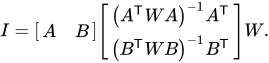
直交条件が 非特異に拡張された場合、次のことが成り立ちます
。
A
T
W
B
=
A
T
W
T
B
=
0
{\displaystyle A^{\mathsf {T}}WB=A^{\mathsf {T}}W^{\mathsf {T}}B=0}
W
{\displaystyle W}
I
=
[
A
B
]
[
(
A
T
W
A
)
−
1
A
T
(
B
T
W
B
)
−
1
B
T
]
W
.
{\displaystyle I={\begin{bmatrix}A&B\end{bmatrix}}{\begin{bmatrix}\left(A^{\mathsf {T}}WA\right)^{-1}A^{\mathsf {T}}\\\left(B^{\mathsf {T}}WB\right)^{-1}B^{\mathsf {T}}\end{bmatrix}}W.}
これらの公式はすべて、転置の代わりに共役転置 が使用されるという条件で、複素内積空間にも当てはまります 。射影和の詳細については、BanerjeeとRoy(2014)を参照してください。 [9] また、基本的な 球面三角法 における射影和の応用については、Banerjee(2004) [10] を参照してください。
斜め投影 斜投影 という用語は 、非直交投影を指すために使用されることがあります。これらの投影は、2 次元の図面で空間図形を表すためにも使用されます ( 斜投影を 参照) が、直交投影ほど頻繁ではありません。 通常の最小二乗回帰の適合値を計算するには直交投影が必要ですが、 操作変数回帰 の適合値を計算するには 斜投影が必要です。
投影は、そのカーネルと、その範囲を特徴付けるために使用される基底ベクトル (カーネルの補完) によって定義されます。これらの基底ベクトルがカーネルに直交する場合、投影は直交投影です。これらの基底ベクトルがカーネルに直交しない場合、投影は斜投影、または単なる投影です。
を となる線形演算子とし 、 は ゼロ演算子ではないと仮定します。ベクトルが の範囲の基底を形成し 、これらのベクトルを 行列にまとめるとします 。 そうでない場合は となり、 は ゼロ演算子となります。範囲と核は相補空間であるため、核の次元は となります 。したがって、 核の 直交補元 の次元は となります。が 射影の核の直交補元の基底を形成し、これらのベクトルを行列 にまとめるとします 。すると、射影 (条件 ) は次式で与えられます。
P
:
V
→
V
{\displaystyle P\colon V\to V}
P
2
=
P
{\displaystyle P^{2}=P}
P
{\displaystyle P}
u
1
,
…
,
u
k
{\displaystyle \mathbf {u} _{1},\ldots ,\mathbf {u} _{k}}
P
{\displaystyle P}
n
×
k
{\displaystyle n\times k}
A
{\displaystyle A}
k
≥
1
{\displaystyle k\geq 1}
k
=
0
{\displaystyle k=0}
P
{\displaystyle P}
n
−
k
{\displaystyle n-k}
k
{\displaystyle k}
v
1
,
…
,
v
k
{\displaystyle \mathbf {v} _{1},\ldots ,\mathbf {v} _{k}}
B
{\displaystyle B}
P
{\displaystyle P}
k
≥
1
{\displaystyle k\geq 1}
P
=
A
(
B
T
A
)
−
1
B
T
.
{\displaystyle P=A\left(B^{\mathsf {T}}A\right)^{-1}B^{\mathsf {T}}.}
この表現は、上で示した直交射影の公式を一般化したものである。 [11] [12] この表現の標準的な証明は以下のとおりである。 ベクトル空間 内の任意のベクトルに対して 、 を分解することができる 。ここでベクトル は の像内にあり 、ベクトルは なので 、 は の核内にあり 、核は の零空間である。 言い換えれば、ベクトルは の列空間内にあるので、ある 次元ベクトル に対して となり 、 の構築によりベクトルはを 満たす。 これらの条件をまとめると、 となるベクトルが見つかる 。 行列 および は 構築により フルランクであるため、 -行列 は可逆である。したがって、方程式は ベクトルを与える。 このようにして、 任意のベクトルに対して となり 、したがって となる 。
x
{\displaystyle \mathbf {x} }
V
{\displaystyle V}
x
=
x
1
+
x
2
{\displaystyle \mathbf {x} =\mathbf {x} _{1}+\mathbf {x} _{2}}
x
1
=
P
(
x
)
{\displaystyle \mathbf {x} _{1}=P(\mathbf {x} )}
P
{\displaystyle P}
x
2
=
x
−
P
(
x
)
.
{\displaystyle \mathbf {x} _{2}=\mathbf {x} -P(\mathbf {x} ).}
P
(
x
2
)
=
P
(
x
)
−
P
2
(
x
)
=
0
{\displaystyle P(\mathbf {x} _{2})=P(\mathbf {x} )-P^{2}(\mathbf {x} )=\mathbf {0} }
x
2
{\displaystyle \mathbf {x} _{2}}
P
{\displaystyle P}
A
.
{\displaystyle A.}
x
1
{\displaystyle \mathbf {x} _{1}}
A
,
{\displaystyle A,}
x
1
=
A
w
{\displaystyle \mathbf {x} _{1}=A\mathbf {w} }
k
{\displaystyle k}
w
{\displaystyle \mathbf {w} }
x
2
{\displaystyle \mathbf {x} _{2}}
B
T
x
2
=
0
{\displaystyle B^{\mathsf {T}}\mathbf {x} _{2}=\mathbf {0} }
B
{\displaystyle B}
w
{\displaystyle \mathbf {w} }
B
T
(
x
−
A
w
)
=
0
{\displaystyle B^{\mathsf {T}}(\mathbf {x} -A\mathbf {w} )=\mathbf {0} }
A
{\displaystyle A}
B
{\displaystyle B}
k
{\displaystyle k}
k
×
k
{\displaystyle k\times k}
B
T
A
{\displaystyle B^{\mathsf {T}}A}
B
T
(
x
−
A
w
)
=
0
{\displaystyle B^{\mathsf {T}}(\mathbf {x} -A\mathbf {w} )=\mathbf {0} }
w
=
(
B
T
A
)
−
1
B
T
x
.
{\displaystyle \mathbf {w} =(B^{\mathsf {T}}A)^{-1}B^{\mathsf {T}}\mathbf {x} .}
P
x
=
x
1
=
A
w
=
A
(
B
T
A
)
−
1
B
T
x
{\displaystyle P\mathbf {x} =\mathbf {x} _{1}=A\mathbf {w} =A(B^{\mathsf {T}}A)^{-1}B^{\mathsf {T}}\mathbf {x} }
x
∈
V
{\displaystyle \mathbf {x} \in V}
P
=
A
(
B
T
A
)
−
1
B
T
{\displaystyle P=A(B^{\mathsf {T}}A)^{-1}B^{\mathsf {T}}}
が直交射影である 場合、 を取ることができ 、 となります 。この公式を使用すると、 であることが簡単に確認できます。一般に、ベクトル空間が複素数体上にある場合、 エルミート転置を 使用して、公式 が得られます 。 は 列フル ランクである ため、 の ムーア-ペンローズ逆行列 をで 表すことができることを思い出してください 。
P
{\displaystyle P}
A
=
B
{\displaystyle A=B}
P
=
A
(
A
T
A
)
−
1
A
T
{\displaystyle P=A\left(A^{\mathsf {T}}A\right)^{-1}A^{\mathsf {T}}}
P
=
P
T
{\displaystyle P=P^{\mathsf {T}}}
A
∗
{\displaystyle A^{*}}
P
=
A
(
A
∗
A
)
−
1
A
∗
{\displaystyle P=A\left(A^{*}A\right)^{-1}A^{*}}
A
{\displaystyle A}
A
+
=
(
A
∗
A
)
−
1
A
∗
{\displaystyle A^{+}=(A^{*}A)^{-1}A^{*}}
A
{\displaystyle A}
P
=
A
A
+
{\displaystyle P=AA^{+}}
特異値
I
−
P
{\displaystyle I-P}
も斜射影です。と の特異値は の 正規直交基底 によって計算できます 。
を の正規直交基底とし 、 を の 直交補行列 とします 。 行列の特異値を
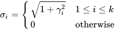
正の値 で表します 。これにより、 の特異値は次のよう になります。 [13]
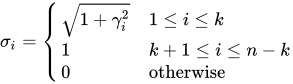
および の特異値は 次のように なります。
これは、 と
の最大特異値が 等しいこと、したがって斜射影の 行列ノルム が同じであることを意味します。ただし、 条件数は という関係を満たすため 、必ずしも等しいとは限りません。
P
{\displaystyle P}
I
−
P
{\displaystyle I-P}
A
{\displaystyle A}
Q
A
{\displaystyle Q_{A}}
A
{\displaystyle A}
Q
A
⊥
{\displaystyle Q_{A}^{\perp }}
Q
A
{\displaystyle Q_{A}}
Q
A
T
A
(
B
T
A
)
−
1
B
T
Q
A
⊥
{\displaystyle Q_{A}^{T}A(B^{T}A)^{-1}B^{T}Q_{A}^{\perp }}
γ
1
≥
γ
2
≥
…
≥
γ
k
{\displaystyle \gamma _{1}\geq \gamma _{2}\geq \ldots \geq \gamma _{k}}
P
{\displaystyle P}
σ
i
=
{
1
+
γ
i
2
1
≤
i
≤
k
0
otherwise
{\displaystyle \sigma _{i}={\begin{cases}{\sqrt {1+\gamma _{i}^{2}}}&1\leq i\leq k\\0&{\text{otherwise}}\end{cases}}}
I
−
P
{\displaystyle I-P}
σ
i
=
{
1
+
γ
i
2
1
≤
i
≤
k
1
k
+
1
≤
i
≤
n
−
k
0
otherwise
{\displaystyle \sigma _{i}={\begin{cases}{\sqrt {1+\gamma _{i}^{2}}}&1\leq i\leq k\\1&k+1\leq i\leq n-k\\0&{\text{otherwise}}\end{cases}}}
P
{\displaystyle P}
I
−
P
{\displaystyle I-P}
κ
(
I
−
P
)
=
σ
1
1
≥
σ
1
σ
k
=
κ
(
P
)
{\displaystyle \kappa (I-P)={\frac {\sigma _{1}}{1}}\geq {\frac {\sigma _{1}}{\sigma _{k}}}=\kappa (P)}
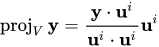
内積による射影の求め方 を直交ベクトルが張るベクトル空間(この場合は平面)とします 。 を ベクトルとします。 の射影を と定義すると 、 繰り返し
の添え字が にわたって合計されます( アインシュタインの和の表記 )。 ベクトルは 、 となる直交和として書くことができます 。は と表記されることもあります。線型代数には、これが からへの 最小距離( 直交距離 )である という定理があり、 機械学習 などの分野でよく使用されます 。
V
{\displaystyle V}
u
1
,
u
2
,
…
,
u
p
{\displaystyle \mathbf {u} _{1},\mathbf {u} _{2},\dots ,\mathbf {u} _{p}}
y
{\displaystyle y}
y
{\displaystyle \mathbf {y} }
V
{\displaystyle V}
proj
V
y
=
y
⋅
u
i
u
i
⋅
u
i
u
i
{\displaystyle \operatorname {proj} _{V}\mathbf {y} ={\frac {\mathbf {y} \cdot \mathbf {u} ^{i}}{\mathbf {u} ^{i}\cdot \mathbf {u} ^{i}}}\mathbf {u} ^{i}}
y
{\displaystyle \mathbf {y} }
y
=
proj
V
y
+
z
{\displaystyle \mathbf {y} =\operatorname {proj} _{V}\mathbf {y} +\mathbf {z} }
proj
V
y
{\displaystyle \operatorname {proj} _{V}\mathbf {y} }
y
^
{\displaystyle {\hat {\mathbf {y} }}}
z
{\displaystyle \mathbf {z} }
y
{\displaystyle \mathbf {y} }
V
{\displaystyle V}
y は ベクトル空間 V に投影されます。
次元 のベクトル空間上の任意の 射影は、 体上では 対角化可能な行列 である 。なぜなら、その 最小多項式は を割り切り 、 は異なる線形因子に分割されるからである。したがって、 の基底が存在し、その基底は次の 形式を持つ。
P
=
P
2
{\displaystyle P=P^{2}}
d
{\displaystyle d}
x
2
−
x
{\displaystyle x^{2}-x}
P
{\displaystyle P}
P
=
I
r
⊕
0
d
−
r
{\displaystyle P=I_{r}\oplus 0_{d-r}}
ここで は の 階数 です 。ここで は サイズ の 単位行列 、 は サイズ の 零行列 、 は 直和演算 子です 。ベクトル空間が複素数で内積 を備えている場合 、 P の行列 が [14]となる 正規直交 基底があります。
r
{\displaystyle r}
P
{\displaystyle P}
I
r
{\displaystyle I_{r}}
r
{\displaystyle r}
0
d
−
r
{\displaystyle 0_{d-r}}
d
−
r
{\displaystyle d-r}
⊕
{\displaystyle \oplus }
P
=
[
1
σ
1
0
0
]
⊕
⋯
⊕
[
1
σ
k
0
0
]
⊕
I
m
⊕
0
s
.
{\displaystyle P={\begin{bmatrix}1&\sigma _{1}\\0&0\end{bmatrix}}\oplus \cdots \oplus {\begin{bmatrix}1&\sigma _{k}\\0&0\end{bmatrix}}\oplus I_{m}\oplus 0_{s}.}
ここで 、 整数 と実数は 一意に決定されます。 因子は、が 直交 射影として作用する 最大不変部分空間に対応し (したがって、 P 自体が直交するのは の場合のみ )、 -ブロックは 斜 交成分に対応します 。
σ
1
≥
σ
2
≥
⋯
≥
σ
k
>
0
{\displaystyle \sigma _{1}\geq \sigma _{2}\geq \dots \geq \sigma _{k}>0}
k
,
s
,
m
{\displaystyle k,s,m}
σ
i
{\displaystyle \sigma _{i}}
2
k
+
s
+
m
=
d
{\displaystyle 2k+s+m=d}
I
m
⊕
0
s
{\displaystyle I_{m}\oplus 0_{s}}
P
{\displaystyle P}
k
=
0
{\displaystyle k=0}
σ
i
{\displaystyle \sigma _{i}}
ノルムベクトル空間への射影 基礎となるベクトル空間 が(必ずしも有限次元ではない) ノルムベクトル空間 である場合、有限次元の場合には無関係な解析的な問題を考慮する必要があります。 が バナッハ空間 であると仮定します 。
X
{\displaystyle X}
X
{\displaystyle X}
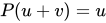
上で議論した代数的結果の多くは、この文脈に移ってもそのまま残っています。 を 相補的な部分空間に直和分解すると、依然として射影が指定され、逆もまた同様です。 が直和 である場合 、 によって定義される演算子は、依然として範囲 と核 を 持つ射影です 。 であることも明らかです 。逆に、 が への射影である場合 、すなわち である場合、 であることが簡単に確認できます 。言い換えると、 も射影です。 関係式は 、 および が 直和 であることを 意味します 。
X
{\displaystyle X}
X
{\displaystyle X}
X
=
U
⊕
V
{\displaystyle X=U\oplus V}
P
(
u
+
v
)
=
u
{\displaystyle P(u+v)=u}
U
{\displaystyle U}
V
{\displaystyle V}
P
2
=
P
{\displaystyle P^{2}=P}
P
{\displaystyle P}
X
{\displaystyle X}
P
2
=
P
{\displaystyle P^{2}=P}
(
1
−
P
)
2
=
(
1
−
P
)
{\displaystyle (1-P)^{2}=(1-P)}
1
−
P
{\displaystyle 1-P}
P
2
=
P
{\displaystyle P^{2}=P}
1
=
P
+
(
1
−
P
)
{\displaystyle 1=P+(1-P)}
X
{\displaystyle X}
rg
(
P
)
⊕
rg
(
1
−
P
)
{\displaystyle \operatorname {rg} (P)\oplus \operatorname {rg} (1-P)}
しかし、有限次元の場合とは対照的に、射影は 一般に 連続で ある必要はありません。 の部分空間が ノルム位相で閉じていない場合、 への射影は 連続ではありません。言い換えると、連続射影の値域は 閉じた部分空間でなければなりません。さらに、連続射影の核(実際には、一般に連続線型演算子)は閉じています。したがって、 連続 射影はを 2 つの相補的な 閉じた 部分空間 に 分解します 。
U
{\displaystyle U}
X
{\displaystyle X}
U
{\displaystyle U}
P
{\displaystyle P}
P
{\displaystyle P}
X
{\displaystyle X}
X
=
rg
(
P
)
⊕
ker
(
P
)
=
ker
(
1
−
P
)
⊕
ker
(
P
)
{\displaystyle X=\operatorname {rg} (P)\oplus \ker(P)=\ker(1-P)\oplus \ker(P)}
逆もまた成り立ちますが、仮定が 1 つ追加されます。 が の閉部分空間であるとします。 X = U ⊕ V となる 閉部分空間が存在する場合、 値域 と核を持つ 射影は 連続です。これは、 閉グラフ定理 から導かれます。 x n → x および Px n → y であるとします。 を示す必要があります 。 は閉じており、 { Px n } ⊂ U であるため、 y は 、すなわち Py = y に含まれます 。また、 x n − Px n = ( I − P ) x n → x − y です。 は閉じており、 {( I − P ) x n } ⊂ V であるため、 、すなわち となり 、主張が証明されます。
U
{\displaystyle U}
X
{\displaystyle X}
V
{\displaystyle V}
P
{\displaystyle P}
U
{\displaystyle U}
V
{\displaystyle V}
P
x
=
y
{\displaystyle Px=y}
U
{\displaystyle U}
U
{\displaystyle U}
V
{\displaystyle V}
x
−
y
∈
V
{\displaystyle x-y\in V}
P
(
x
−
y
)
=
P
x
−
P
y
=
P
x
−
y
=
0
{\displaystyle P(x-y)=Px-Py=Px-y=0}
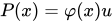
上記の議論は、と が 両方とも閉じているという仮定を利用しています 。一般に、閉部分空間 が与えられた場合 、相補閉部分空間 が存在する必要はありませ んが、 ヒルベルト空間の場合は、 直交相補 を 取ることで常にこれを行うことができます 。バナッハ空間の場合、1 次元部分空間には必ず閉じた相補部分空間があります。これは、 ハーン・バナッハの定理 から直接導かれる結果です。 を の線型スパンとします。ハーン・バナッハの定理により、 φ ( u ) = 1 となる有界 線型汎関数 が存在します 。演算子 はを 満たします 。つまり、これは射影です。 が有界であることは の連続性を意味し 、したがって は の閉じた相補部分空間です 。
U
{\displaystyle U}
V
{\displaystyle V}
U
{\displaystyle U}
V
{\displaystyle V}
U
{\displaystyle U}
u
{\displaystyle u}
φ
{\displaystyle \varphi }
P
(
x
)
=
φ
(
x
)
u
{\displaystyle P(x)=\varphi (x)u}
P
2
=
P
{\displaystyle P^{2}=P}
φ
{\displaystyle \varphi }
P
{\displaystyle P}
ker
(
P
)
=
rg
(
I
−
P
)
{\displaystyle \ker(P)=\operatorname {rg} (I-P)}
U
{\displaystyle U}
アプリケーションとさらなる検討 投影(直交投影など)は、 特定の線形代数問題の
アルゴリズムで重要な役割を果たします。
上で述べたように、射影は冪等性の特殊なケースです。解析的には、直交射影は 特性関数 の非可換な一般化です。冪等性は、例えば 半単純代数の 分類に使用され、 測度論は 測定可能な集合 の特性関数を考慮することから始まります 。したがって、想像できるように、射影は 作用素代数 の文脈で非常に頻繁に遭遇します。特に、 フォン ノイマン代数は、射影の完全な 格子 によって生成されます 。
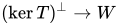
一般化 より一般的には、ノルムベクトル空間間の写像が与えられた場合 、同様にこの写像が核の直交補写像上の等長写像となるように求めることができます。つまり、 は等長写像( 部分等長写像 を参照 )である必要があります。特に、 は 上に なければなりません。直交射影の場合は、 W が V の部分空間である場合です。 リーマン幾何学 では、これは リーマン沈み込み の定義で使用されます 。
T
:
V
→
W
,
{\displaystyle T\colon V\to W,}
(
ker
T
)
⊥
→
W
{\displaystyle (\ker T)^{\perp }\to W}
参照
注記
^ マイヤー、pp 386+387 ^ ab Horn, Roger A.; Johnson, Charles R. (2013). Matrix Analysis, 第 2 版 . Cambridge University Press. ISBN 9780521839402 。 ^ マイヤー、433ページ ^ マイヤー、431ページ ^ マイヤー、式 (5.13.4) ^ Banerjee, Sudipto; Roy, Anindya (2014)、統計のための線形代数と行列分析、統計科学テキスト(第1版)、Chapman and Hall/CRC、 ISBN 978-1420095388 ^ マイヤー、式 (5.13.3) ^ 線形最小二乗法 (数学) § 最小二乗推定量の性質 も参照してください 。 ^ Banerjee, Sudipto; Roy, Anindya (2014)、統計のための線形代数と行列分析、統計科学テキスト(第1版)、Chapman and Hall/CRC、 ISBN 978-1420095388 ^ Banerjee, Sudipto (2004)、「直交投影法による球面三角法の再検討」、 The College Mathematics Journal 、 35 (5): 375–381、 doi :10.1080/07468342.2004.11922099、 S2CID 122277398 ^ Banerjee, Sudipto; Roy, Anindya (2014)、統計のための線形代数と行列分析、統計科学テキスト(第1版)、Chapman and Hall/CRC、 ISBN 978-1420095388 ^ マイヤー、方程式 (7.10.39) ^ Brust, JJ; Marcia, RF; Petra, CG (2020)、「斜投影行列の計算効率の良い分解」、 SIAM Journal on Matrix Analysis and Applications 、 41 (2): 852–870、 doi :10.1137/19M1288115、 OSTI 1680061、 S2CID 219921214 ^ ドコヴィッチ、D. Ž. (1991年8月)。 「プロジェクターの単一類似性」。 数学の方程式 。 42 (1): 220–224。 土井 :10.1007/BF01818492。 S2CID 122704926。
参考文献 Banerjee, Sudipto; Roy, Anindya (2014)、 「統計のための線形代数と行列分析」 、Texts in Statistical Science (第 1 版)、Chapman and Hall/CRC、 ISBN 978-1420095388 Dunford, N.; Schwartz, JT (1958). 線形演算子、パート I: 一般理論 . インターサイエンス。 マイヤー、カール D. (2000)。行列解析と応用線形代数。工業応用数学協会 。ISBN 978-0-89871-454-8 。
外部リンク
























































![{\displaystyle {\begin{aligned}I&={\begin{bmatrix}A&B\end{bmatrix}}{\begin{bmatrix}A&B\end{bmatrix}}^{-1}{\begin{bmatrix}A^{\mathsf {T}}\\B^{\mathsf {T}}\end{bmatrix}}^{-1}{\begin{bmatrix}A^{\mathsf {T}}\\B^{\mathsf {T}}\end{bmatrix}}\\&={\begin{bmatrix}A&B\end{bmatrix}}\left({\begin{bmatrix}A^{\mathsf {T}}\\B^{\mathsf {T}}\end{bmatrix}}{\begin{bmatrix}A&B\end{bmatrix}}\right)^{-1}{\begin{bmatrix}A^{\mathsf {T}}\\B^{\mathsf {T}}\end{bmatrix}}\\&={\begin{bmatrix}A&B\end{bmatrix}}{\begin{bmatrix}A^{\mathsf {T}}A&O\\O&B^{\mathsf {T}}B\end{bmatrix}}^{-1}{\begin{bmatrix}A^{\mathsf {T}}\\B^{\mathsf {T}}\end{bmatrix}}\\[4pt]&=A\left(A^{\mathsf {T}}A\right)^{-1}A^{\mathsf {T}}+B\left(B^{\mathsf {T}}B\right)^{-1}B^{\mathsf {T}}\end{aligned}}}](https://wikimedia.org/api/rest_v1/media/math/render/svg/0d5ac3d05451825c162acf531a9416503f4a580e)