The transition probability, the probability of going from to , is introduced here; the expectation can be written as Now we replace in the definition of , multiply by and integrate over . The limit is taken on Note now that which is the Chapman–Kolmogorov theorem. Changing the dummy variable to , one gets which is a time derivative. Finally we arrive to From here, the Kolmogorov backward equation can be deduced. If we instead use the adjoint operator of , , defined such that then we arrive to the Kolmogorov forward equation, or Fokker–Planck equation, which, simplifying the notation , in its differential form reads
Remains the issue of defining explicitly . This can be done taking the expectation from the integral form of the Itô's lemma:
The part that depends on vanished because of the martingale property.
Then, for a particle subject to an Itô equation, using it can be easily calculated, using integration by parts, that which bring us to the Fokker–Planck equation:
The Fokker–Planck equation is used with problems where the initial distribution is known. If, instead, a final point is fixed, the Feynman–Kac formula can be used to calculate expectation values such as mean first-passage times, which is a consequence of the Kolmogorov backward equation. If the problem is to know the distribution at previous times, starting from a known distribution at later times, a reverse-time Fokker-Planck equation can be constructed.[11]
The stochastic process defined above in the Itô sense can be rewritten within the Stratonovich convention as a Stratonovich SDE: It includes an added noise-induced drift term due to diffusion gradient effects if the noise is state-dependent. This convention is more often used in physical applications. Indeed, it is well known that any solution to the Stratonovich SDE is a solution to the Itô SDE.
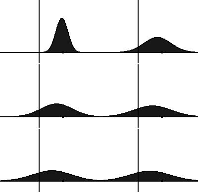
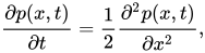
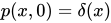
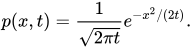
The zero-drift equation with constant diffusion can be considered as a model of classical Brownian motion:
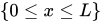
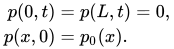
This model has discrete spectrum of solutions if the condition of fixed boundaries is added for :
It has been shown[12] that in this case an analytical spectrum of solutions allows deriving a local uncertainty relation for the coordinate-velocity phase volume: Here 対応する拡散スペクトルの最小値である、 その間そして座標と速度の定義における不確実性を表す。
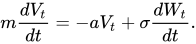
Brownian motion follows the Langevin equation, which can be solved for many different stochastic forcings with results being averaged (canonical ensemble in molecular dynamics). However, instead of this computationally intensive approach, one can use the Fokker–Planck equation and consider the probability of the particle having a velocity in the interval when it starts its motion with at time0.
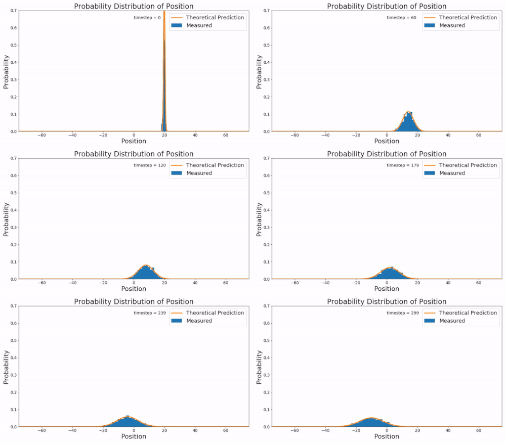
Brownian dynamics simulation for particles in 1-D linear potential compared with the solution of the Fokker–Planck equation
1-D linear potential example
Brownian dynamics in one dimension is simple.[15][16]
Theory
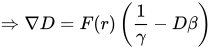
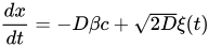
Starting with a linear potential of the form the corresponding Smoluchowski equation becomes,
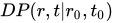
where the diffusion constant, , is constant over space and time. The boundary conditions are such that the probability vanishes at with an initial condition of the ensemble of particles starting in the same place, .
Defining and and applying the coordinate transformation,
With the Smoluchowki equation becomes,
which is the free diffusion equation with solution,
And after transforming back to the original coordinates,
Simulation
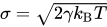
The simulation on the right was completed using a Brownian dynamics simulation.[17][18] Starting with a Langevin equation for the system, where is the friction term, is a fluctuating force on the particle, and is the amplitude of the fluctuation. At equilibrium the frictional force is much greater than the inertial force, . Therefore, the Langevin equation becomes,
For the Brownian dynamic simulation the fluctuation force is assumed to be Gaussian with the amplitude being dependent of the temperature of the system . Rewriting the Langevin equation,
where is the Einstein relation. The integration of this equation was done using the Euler–Maruyama method to numerically approximate the path of this Brownian particle.
↑コルモゴロフ、アンドレイ (1931)。 "Über die Analytischen Methoden in der Wahrscheinlichkeitstheorie" [確率論における分析手法について] Mathematische Annalen (ドイツ語)。104 (1): 415–458 [pp. 448–451]。土井:10.1007/BF01457949。S2CID 119439925。
↑ Dhont, JKG (1996). 『コロイドの動力学入門』 Elsevier. p. 183. ISBN978-0-08-053507-4。
↑ Paul, Wolfgang; Baschnagel, Jörg (2013). "確率論の数学に関する簡潔な概説". Stochastic Processes . Springer. pp. 17–61 [特に33–35]. doi : 10.1007/978-3-319-00327-6_2 . ISBN978-3-319-00326-9。
↑N. N. Bogolyubov Jr. and D. P. Sankovich (1994). "N. N. Bogolyubov and statistical mechanics". Russian Math. Surveys49(5): 19—49. doi:10.1070/RM1994v049n05ABEH002419
↑N. N. Bogoliubov and N. M. Krylov (1939). Fokker–Planck equations generated in perturbation theory by a method based on the spectral properties of a perturbed Hamiltonian. Zapiski Kafedry Fiziki Akademii Nauk Ukrainian SSR 4: 81–157 (in Ukrainian).
↑Risken, H. (1996), The Fokker–Planck Equation: Methods of Solution and Applications, vol.Second Edition, Third Printing, p.72
12Öttinger, Hans Christian (1996). Stochastic Processes in Polymeric Fluids. Berlin-Heidelberg: Springer-Verlag. p.75. ISBN978-3-540-58353-0.
↑Anderson, Brian D. O. (1982-05-01). "Reverse-time diffusion equation models". Stochastic Processes and their Applications. 12 (3): 313–326. doi:10.1016/0304-4149(82)90051-5. ISSN0304-4149.
↑Kamenshchikov, S. (2014). "Clustering and Uncertainty in Perfect Chaos Systems". Journal of Chaos. 2014: 1–6. arXiv:1301.4481. doi:10.1155/2014/292096. S2CID17719673.
↑Pavliotis, Grigorios A. (2014). Stochastic Processes and Applications: Diffusion Processes, the Fokker-Planck and Langevin Equations. Springer. pp.38–40. doi:10.1007/978-1-4939-1323-7_2. ISBN978-1-4939-1322-0.
↑Rosenbluth, M. N. (1957). "Fokker–Planck Equation for an Inverse-Square Force". Physical Review. 107 (1): 1–6. Bibcode:1957PhRv..107....1R. doi:10.1103/physrev.107.1.
↑ Janssen, HK (1976). "On a Lagrangean for Classical Field Dynamics and Renormalization Group Calculation of Dynamical Critical Properties". Z. Phys . B23 (4): 377–380 . Bibcode : 1976ZPhyB..23..377J . doi : 10.1007/BF01316547 . S2CID 121216943 .
さらに読む
Frank, Till Daniel (2005).非線形フォッカー・プランク方程式:基礎と応用. Springer Series in Synergetics. Springer. ISBN3-540-21264-7。







![{\displaystyle {\frac {\partial }{\partial t}}p(x,t)=-{\frac {\partial }{\partial x}}\left[\mu (x,t)p(x,t)\right]+{\frac {\partial ^{2}}{\partial x^{2}}}\left[D(x,t)p(x,t)\right].}](https://wikimedia.org/api/rest_v1/media/math/render/svg/8f66f454692d4179f5de829965a2237a65485940)


![{\displaystyle {\mathcal {L}}p(X_{t})=\lim _{\Delta t\to 0}{\frac {1}{\Delta t}}\left(\mathbb {E} {\big [}p(X_{t+\Delta t})\mid X_{t}=x{\big ]}-p(x)\right).}](https://wikimedia.org/api/rest_v1/media/math/render/svg/fbbac0ac010adeabfb6a94014fcae99d7f637597)









![\displaystyle \int [{\mathcal {L}}p(x)]\mathbb {P} _{t,t'}(x\mid x')\,dx=\int p(x)\,{\frac {\partial }{\partial t}}\mathbb {P} _{t,t'}(x\mid x')\,dx.}](https://wikimedia.org/api/rest_v1/media/math/render/svg/fc1023c90d752868d7120ac3a803568153fc9369)

![{\displaystyle \int [{\mathcal {L}}p(x)]\mathbb {P} _{t,t'}(x\mid x')\,dx=\int p(x)[{\mathcal {L}}^{\dagger }\mathbb {P} _{t,t'}(x\mid x')]\,dx,}](https://wikimedia.org/api/rest_v1/media/math/render/svg/6d792d0f77b1cb0bdb5b405ed785eb3bda1873b3)



![{\displaystyle dX_{t}=\left[\mu (X_{t},t)-{\frac {1}{2}}{\frac {\partial }{\partial X_{t}}}D(X_{t},t)\right]\,dt+{\sqrt {2D(X_{t},t)}}\circ dW_{t}.}](https://wikimedia.org/api/rest_v1/media/math/render/svg/74f54b781333612a077d5fc2cb0f91f8f7fe60f2)
![${\displaystyle {\frac {\partial }{\partial t}}p(x,t)=D_{0}{\frac {\partial ^{2}}{\partial x^{2}}}\left[p(x,t)\right].}$](https://wikimedia.org/api/rest_v1/media/math/render/svg/1c9029fd21c2e3e7258c6d6c08f64914193bbbf6)






![{\displaystyle {\frac {\partial p(\mathbf {x} ,t)}{\partial t}}=-\sum _{i=1}^{N}{\frac {\partial }{\partial x_{i}}}\left[\mu _{i}(\mathbf {x} ,t)p(\mathbf {x} ,t)\right]+\sum _{i=1}^{N}\sum _{j=1}^{N}{\frac {\partial ^{2}}{\partial x_{i}\,\partial x_{j}}}\left[D_{ij}(\mathbf {x} ,t)p(\mathbf {x} ,t)\right],}](https://wikimedia.org/api/rest_v1/media/math/render/svg/75b4e22a5e4eff2c83ea5895484ee1fb39cf5ea5)


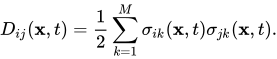

![{\displaystyle {\frac {\partial p(\mathbf {x} ,t)}{\partial t}}=-\sum _{i=1}^{N}{\frac {\partial }{\partial x_{i}}}\left[\mu _{i}(\mathbf {x} ,t)\,p(\mathbf {x} ,t)\right]+{\frac {1}{2}}\sum _{k=1}^{M}\sum _{i=1}^{N}{\frac {\partial }{\partial x_{i}}}\left\{\sigma _{ik}(\mathbf {x} ,t)\sum _{j=1}^{N}{\frac {\partial }{\partial x_{j}}}\left[\sigma _{jk}(\mathbf {x} ,t)\,p(\mathbf {x} ,t)\right]\right\}}](https://wikimedia.org/api/rest_v1/media/math/render/svg/66bb0ebd3cce662da5ddb4f025d1f08ab0a0b15c)























![{\displaystyle {\frac {\partial }{\partial t}}P(r,t\mid r_{0},t_{0})=\nabla \cdot \left[D\left(\nabla -\beta F(r)\right)P(r,t\mid r_{0},t_{0})\right]}](https://wikimedia.org/api/rest_v1/media/math/render/svg/c909422104778d4ee87332685591d39aace6efda)











![{\displaystyle P(x,t\mid x_{0},t_{0})={\frac {1}{\sqrt {4\pi D(t-t_{0})}}}\exp {\left[{-{\frac {\left(x-x_{0}+D\beta c\left(t-t_{0}\right)\right)^{2}}{4D\left(t-t_{0}\right)}}}\right]}}](https://wikimedia.org/api/rest_v1/media/math/render/svg/9e84e888b0f40914f4ffdc698b92c0f912eb20e1)






![{\displaystyle {\begin{aligned}{\frac {\partial }{\partial t}}p{\left(x',t\right)}&=-{\frac {\partial }{\partial x'}}\left[D_{1}(x',t)p(x',t)\right]+{\frac {\partial ^{2}}{\partial {x'}^{2}}}\left[D_{2}(x',t)p(x',t)\right]\\[1ex]&=\int _{-\infty }^{\infty }dx\left[\left(D_{1}{\left(x,t\right)}{\frac {\partial }{\partial x}}+D_{2}{\left(x,t\right)}{\frac {\partial ^{2}}{\partial x^{2}}}\right)\delta {\left(x'-x\right)}\right]p(x,t).\end{aligned}}}](https://wikimedia.org/api/rest_v1/media/math/render/svg/2e49bbee6166c71d0810f99a5e2f171c0cd77fc2)


![{\displaystyle p(x',t{+}\varepsilon )=\int _{-\infty }^{\infty }\,dx\left[\left(1+\varepsilon D_{1}(x,t){\frac {\partial }{\partial x}}+\varepsilon D_{2}(x,t){\frac {\partial ^{2}}{\partial x^{2}}}\right)\delta (x'-x)\right]p(x,t)+O(\varepsilon ^{2}).}](https://wikimedia.org/api/rest_v1/media/math/render/svg/dc1cac92abfc29e28fcc28ab30eb60aa82a58ee6)
![{\displaystyle {\begin{aligned}p(x',t+\varepsilon )&=\int _{-\infty }^{\infty }dx\int _{-i\infty }^{i\infty }{\frac {d{\tilde {x}}}{2\pi i}}\left(1+\varepsilon \left[{\tilde {x}}D_{1}(x,t)+{\tilde {x}}^{2}D_{2}(x,t)\right]\right)e^{{\tilde {x}}(xx')}p(x,t)+O(\varepsilon ^{2})\\[5pt]&=\int _{-\infty }^{\infty }dx\int _{-i\infty }^{i\infty }{\frac {d{\tilde {x}}}{2\pi i}}\exp \left(\varepsilon \left[-{\tilde {x}}{\frac {(x'-x)}{\varepsilon }}+{\tilde {x}}D_{1}(x,t)+{\tilde {x}}^{2}D_{2}(x,t)\right]\right)p(x,t)+O(\varepsilon ^{2}).\end{aligned}}}](https://wikimedia.org/api/rest_v1/media/math/render/svg/5799d4e49249a1a625afdab3bb13ba453e448647)


![{\displaystyle S=\int dt\left[{\tilde {x}}D_{1}(x,t)+{\tilde {x}}^{2}D_{2}(x,t)-{\tilde {x}}{\frac {\partial x}{\partial t}}\right].}](https://wikimedia.org/api/rest_v1/media/math/render/svg/b385884d6d5ef443c5f67e98c62ae45e29f43e00)
