sin、cos、tan などの逆関数。
数学 において 、 逆三角関数( 逆三角関数 [1] 、 循環 関数 [2] 、 または 弧 関数 [3] とも呼ばれる )は、適切に制限された定義 域 における 三角関数 の 逆関数である。具体的には、 正弦関数 、 余弦関数 、 正接 関数、 余接関数 、 割線関数 、 余割 関数 の逆関数であり [4] 、任意の角度の三角比から角度を取得するために使用される。逆三角関数は、 工学 、 航海 、 物理学 、 幾何学 で広く使用されている。
表記 半径 1 の円の場合、arcsin と arccos は、問題の量によって決定される実際の円弧の長さです。 逆三角関数の表記法はいくつかあります。最も一般的な慣例は、逆三角関数に arc- 接頭辞を使用して名前を付けることです。arcsin ( x ) 、 arccos( x ) 、 arctan( x ) などです。 [1] (この表記法はこの記事全体で使用されます。) この表記法は、次の幾何学的関係から生じています。 [ 要出典 ]
ラジアンで測定する場合、角度 θラジアンは、長さが rθ の 円弧 に対応します。 ここで、 r は円の半径です。したがって、 単位円 では、 x の余弦関数は円弧と角度の両方です。これは、半径 1 の円弧が角度と同じだからです。または、「余弦が xである円弧」は「余弦が x である角度」と同じです 。これは、円弧の半径での長さが、角度のラジアンでの測定値と同じだからです。 [5] コンピュータプログラミング言語では、逆三角関数は asin 、 acos 、 atanなど の省略形で呼ばれることが多い。 [6]
1813 年に ジョン・ハーシェル によって導入された sin −1 ( x ) 、 cos −1 ( x ) 、 tan −1 ( x ) などの表記法 [7] [8]は、英語の文献 [1] でもよく使われており、同じく 確立された sin [−1] ( x ) 、 cos [−1] ( x ) 、 tan [−1] ( x ) よりもはるかに多く使用されています。これらは、逆関数の表記法と一貫性のある慣習であり、たとえば、各逆三角関数の多値バージョンを定義するのに役立ちます。ただし、これは sin 2 ( x ) など の 式 の 一般 的 な 意味 論 と 論理 的に矛盾しているように見えるかもしれませんが (ただし、括弧なしの sin 2 x だけが実際によく使用されます)、これらの式は関数の合成ではなく数値の累乗を参照するため、逆数 ( 乗法逆数 ) と 逆関数 の表記法が混同される可能性があります 。 [9]
tan
−
1
(
x
)
=
{
arctan
(
x
)
+
π
k
∣
k
∈
Z
}
.
{\displaystyle \tan ^{-1}(x)=\{\arctan(x)+\pi k\mid k\in \mathbb {Z} \}~.}
逆三角関数にはそれぞれ独自の名前が付いているため、混乱はある程度緩和されます。たとえば、 (cos( x )) −1 = sec( x ) などです。ただし、あいまいであるため、この関数を使用しないよう推奨する著者もいます。 [1] [10] 少数の著者によって使用されている別の危うい慣例に 、最初の文字を 大文字にして上付き文字「 −1 」を使用するものがあります。 Sin −1 ( x ) 、 Cos −1 ( x ) 、 Tan −1 ( x ) などです。 [11] これは、 逆数との混同を避けるためのもので、逆数は sin −1 ( x ) 、 cos −1 ( x ) など、またはより適切なのは sin −1 x 、 cos −1 x などと表されるべきです が、多くの一般的な高水準プログラミング言語(例: Mathematica や MAGMA )が標準の三角関数にまったく同じ大文字の表現を使用しているのに対し、他の言語( Python 、 SymPy 、 NumPy 、 Matlab 、 MAPLE など)は小文字を使用しているため、今度は大きな曖昧さの原因となります。
したがって、2009 年以降、 ISO 80000-2 規格では、逆関数に対して「arc」接頭辞のみが指定されています。
基本概念 1 、 Sec( θ ) 、 Csc( θ ) とラベル付けされた点は、 原点からその点までの線分の長さを表します。Sin ( θ ) 、 Tan( θ ) 、 1は、 x 軸から始まる線分の高さであり 、 Cos( θ ) 、 1 、 Cot( θ )は、原点から始まる x 軸に沿った長さです 。
主な価値観 6 つの三角関数はいずれも 1 対 1 ではないため、逆関数を持つためには制限が必要です。したがって、逆関数の結果の 範囲は、 元の関数の定義域の適切な (つまり厳密な) サブセット になります。
たとえば、 関数 を 多価関数 の意味で使用する場合、 平方根 関数は から定義できるの と同じように、 関数 は となる ように定義されます。 となる実数が与えられた場合、 となる数 が複数(実際には、 可算無限個 )存在します 。たとえば、となるだけ でなく、 となる数も存在します 。 値が 1 つだけ必要な場合は、関数をその 主枝 に制限することができます。この制限により、 ドメイン内の のそれぞれについて、式は という単一の値のみに評価されます 。 これらの特性は、すべての逆三角関数に適用されます。
y
=
x
{\displaystyle y={\sqrt {x}}}
y
2
=
x
,
{\displaystyle y^{2}=x,}
y
=
arcsin
(
x
)
{\displaystyle y=\arcsin(x)}
sin
(
y
)
=
x
.
{\displaystyle \sin(y)=x.}
x
,
{\displaystyle x,}
−
1
≤
x
≤
1
,
{\displaystyle -1\leq x\leq 1,}
y
{\displaystyle y}
sin
(
y
)
=
x
{\displaystyle \sin(y)=x}
sin
(
0
)
=
0
,
{\displaystyle \sin(0)=0,}
sin
(
π
)
=
0
,
{\displaystyle \sin(\pi )=0,}
sin
(
2
π
)
=
0
,
{\displaystyle \sin(2\pi )=0,}
x
{\displaystyle x}
arcsin
(
x
)
{\displaystyle \arcsin(x)}
主な逆関数は次の表に示されています。
注: 一部の著者 [ 要出典 ] は、アークセカントの範囲を と定義しています 。これは、正接関数がこの領域で非負であるためです。これにより、一部の計算がより一貫性を持ちます。たとえば、この範囲を使用すると、 範囲 の場合はと 書く必要があります。 これは、正接関数が では非負です が、 では非正であるためです。 同様の理由で、同じ著者がアークコセカントの範囲を または と定義しています。
(
0
≤
y
<
π
2
or
π
≤
y
<
3
π
2
)
{\textstyle (0\leq y<{\frac {\pi }{2}}{\text{ or }}\pi \leq y<{\frac {3\pi }{2}})}
tan
(
arcsec
(
x
)
)
=
x
2
−
1
,
{\displaystyle \tan(\operatorname {arcsec}(x))={\sqrt {x^{2}-1}},}
(
0
≤
y
<
π
2
or
π
2
<
y
≤
π
)
{\textstyle (0\leq y<{\frac {\pi }{2}}{\text{ or }}{\frac {\pi }{2}}<y\leq \pi )}
tan
(
arcsec
(
x
)
)
=
±
x
2
−
1
,
{\displaystyle \tan(\operatorname {arcsec}(x))=\pm {\sqrt {x^{2}-1}},}
0
≤
y
<
π
2
,
{\textstyle 0\leq y<{\frac {\pi }{2}},}
π
2
<
y
≤
π
.
{\textstyle {\frac {\pi }{2}}<y\leq \pi .}
(
−
π
<
y
≤
−
π
2
{\textstyle (-\pi <y\leq -{\frac {\pi }{2}}}
0
<
y
≤
π
2
)
.
{\textstyle 0<y\leq {\frac {\pi }{2}}).}
ドメイン が複素数 であることが許可されている 場合 、 の範囲は その実数部にのみ適用されます。
x
{\displaystyle x}
y
{\displaystyle y}
以下の表は、逆三角関数の名前と定義域、および それらの通常の 主値の 範囲を ラジアン で示しています 。
記号は 実数 全体の集合を表し 、 は 整数 全体の集合を表します 。 の整数倍全体の集合 は で表されます。
R
=
(
−
∞
,
∞
)
{\displaystyle \mathbb {R} =(-\infty ,\infty )}
Z
=
{
…
,
−
2
,
−
1
,
0
,
1
,
2
,
…
}
{\displaystyle \mathbb {Z} =\{\ldots ,\,-2,\,-1,\,0,\,1,\,2,\,\ldots \}}
π
{\displaystyle \pi }
π
Z
:=
{
π
n
:
n
∈
Z
}
=
{
…
,
−
2
π
,
−
π
,
0
,
π
,
2
π
,
…
}
.
{\displaystyle \pi \mathbb {Z} ~:=~\{\pi n\;:\;n\in \mathbb {Z} \}~=~\{\ldots ,\,-2\pi ,\,-\pi ,\,0,\,\pi ,\,2\pi ,\,\ldots \}.}
記号は 集合減算 を表し 、例えば、は 区間内に ない (つまり実数) の点の集合である。
∖
{\displaystyle \,\setminus \,}
R
∖
(
−
1
,
1
)
=
(
−
∞
,
−
1
]
∪
[
1
,
∞
)
{\displaystyle \mathbb {R} \setminus (-1,1)=(-\infty ,-1]\cup [1,\infty )}
R
{\displaystyle \mathbb {R} }
(
−
1
,
1
)
.
{\displaystyle (-1,1).}
ここで、
の領域を簡潔に記述するために上で使用されている ミンコフスキー 和 表記 法とについて説明します。
π
Z
+
(
0
,
π
)
{\textstyle \pi \mathbb {Z} +(0,\pi )}
π
Z
+
(
−
π
2
,
π
2
)
{\displaystyle \pi \mathbb {Z} +{\bigl (}{-{\tfrac {\pi }{2}}},{\tfrac {\pi }{2}}{\bigr )}}
cot
,
csc
,
tan
,
and
sec
{\displaystyle \cot ,\csc ,\tan ,{\text{ and }}\sec }
コタンジェントとコセカント のドメイン
cot
{\displaystyle \cot }
csc
{\displaystyle \csc }
:と のドメイン は同じです。これらは、 ある整数に対して の 形を とらない すべての実数、 つまりすべての角度の集合です。
cot
{\displaystyle \,\cot \,}
csc
{\displaystyle \,\csc \,}
θ
{\displaystyle \theta }
sin
θ
≠
0
,
{\displaystyle \sin \theta \neq 0,}
π
n
{\displaystyle \pi n}
n
,
{\displaystyle n,}
π
Z
+
(
0
,
π
)
=
⋯
∪
(
−
2
π
,
−
π
)
∪
(
−
π
,
0
)
∪
(
0
,
π
)
∪
(
π
,
2
π
)
∪
⋯
=
R
∖
π
Z
{\displaystyle {\begin{aligned}\pi \mathbb {Z} +(0,\pi )&=\cdots \cup (-2\pi ,-\pi )\cup (-\pi ,0)\cup (0,\pi )\cup (\pi ,2\pi )\cup \cdots \\&=\mathbb {R} \setminus \pi \mathbb {Z} \end{aligned}}}
接線 と割線
tan
{\displaystyle \tan }
sec
{\displaystyle \sec }
の定義域:と の定義域は 同じです。これらは 、
tan
{\displaystyle \,\tan \,}
sec
{\displaystyle \,\sec \,}
θ
{\displaystyle \theta }
cos
θ
≠
0
,
{\displaystyle \cos \theta \neq 0,}
π
Z
+
(
−
π
2
,
π
2
)
=
⋯
∪
(
−
3
π
2
,
−
π
2
)
∪
(
−
π
2
,
π
2
)
∪
(
π
2
,
3
π
2
)
∪
⋯
=
R
∖
(
π
2
+
π
Z
)
{\displaystyle {\begin{aligned}\pi \mathbb {Z} +\left(-{\tfrac {\pi }{2}},{\tfrac {\pi }{2}}\right)&=\cdots \cup {\bigl (}{-{\tfrac {3\pi }{2}}},{-{\tfrac {\pi }{2}}}{\bigr )}\cup {\bigl (}{-{\tfrac {\pi }{2}}},{\tfrac {\pi }{2}}{\bigr )}\cup {\bigl (}{\tfrac {\pi }{2}},{\tfrac {3\pi }{2}}{\bigr )}\cup \cdots \\&=\mathbb {R} \setminus \left({\tfrac {\pi }{2}}+\pi \mathbb {Z} \right)\\\end{aligned}}}
基本的な三角方程式の解 各三角関数は、その引数の実部において周期的であり、各区間ですべての値を2回通過する。
2
π
:
{\displaystyle 2\pi :}
正弦と余弦の周期は ( は整数)で始まり、で終わり、 その後 反転して
2
π
k
−
π
2
{\textstyle 2\pi k-{\frac {\pi }{2}}}
k
{\displaystyle k}
2
π
k
+
π
2
,
{\textstyle 2\pi k+{\frac {\pi }{2}},}
2
π
k
+
π
2
{\textstyle 2\pi k+{\frac {\pi }{2}}}
2
π
k
+
3
π
2
.
{\textstyle 2\pi k+{\frac {3\pi }{2}}.}
コサインとセカントの周期は で始まり、 で終わり 、その後反転して になります。
2
π
k
,
{\displaystyle 2\pi k,}
2
π
k
+
π
.
{\displaystyle 2\pi k+\pi .}
2
π
k
+
π
{\displaystyle 2\pi k+\pi }
2
π
k
+
2
π
.
{\displaystyle 2\pi k+2\pi .}
接線は周期を で開始し、 で終了し、それを まで 繰り返します(前方へ)。
2
π
k
−
π
2
,
{\textstyle 2\pi k-{\frac {\pi }{2}},}
2
π
k
+
π
2
,
{\textstyle 2\pi k+{\frac {\pi }{2}},}
2
π
k
+
π
2
{\textstyle 2\pi k+{\frac {\pi }{2}}}
2
π
k
+
3
π
2
.
{\textstyle 2\pi k+{\frac {3\pi }{2}}.}
コタンジェントの周期は で始まり、 で終了し 、その後 まで繰り返します(順方向) 。
2
π
k
,
{\displaystyle 2\pi k,}
2
π
k
+
π
,
{\displaystyle 2\pi k+\pi ,}
2
π
k
+
π
{\displaystyle 2\pi k+\pi }
2
π
k
+
2
π
.
{\displaystyle 2\pi k+2\pi .}
この周期性は、一般的な逆関数に反映されます。ここでは、 は整数です。
k
{\displaystyle k}
次の表は、6 つの標準三角関数を含む等式を解くために逆三角関数がどのように使用されるかを示しています。指定された値 とは すべて適切な範囲内にあると想定されており、以下の関連する式は 明確に定義されています 。「いくつかの」は「いくつかの 整数 について」
の別の言い方であることに注意してください。
θ
,
{\displaystyle \theta ,}
r
,
{\displaystyle r,}
s
,
{\displaystyle s,}
x
,
{\displaystyle x,}
y
{\displaystyle y}
k
∈
Z
{\displaystyle k\in \mathbb {Z} }
k
.
{\displaystyle k.}
この記号は 論理的等価性を 表し、左辺が真であれば右辺も真であり、逆に右辺が真であれば左辺も真であることを示します (この概念 の 詳細と例については、
この脚注 [注 1]を参照してください)。
⟺
{\displaystyle \,\iff \,}
ここで、最初の 4 つのソリューションは、展開形式で次のように記述できます。
たとえば、 の場合、 ある に対して であり、 の場合 、 ある に対して である場合、 の 場合に は 偶数であり 、 の場合に は奇数です。 方程式および は 、それぞれ および と 同じ解を持ちます 。先ほど解いた方程式 (つまり、 / および / を除く) を 除く 上記のすべての方程式において、解の式の整数 は によって一意に決定されます ( および を固定した場合 )。
cos
θ
=
−
1
{\displaystyle \cos \theta =-1}
θ
=
π
+
2
π
k
=
−
π
+
2
π
(
1
+
k
)
{\displaystyle \theta =\pi +2\pi k=-\pi +2\pi (1+k)}
k
∈
Z
.
{\displaystyle k\in \mathbb {Z} .}
sin
θ
=
±
1
{\displaystyle \sin \theta =\pm 1}
θ
=
π
2
+
π
k
=
−
π
2
+
π
(
k
+
1
)
{\textstyle \theta ={\frac {\pi }{2}}+\pi k=-{\frac {\pi }{2}}+\pi (k+1)}
k
∈
Z
,
{\displaystyle k\in \mathbb {Z} ,}
k
{\displaystyle k}
sin
θ
=
1
{\displaystyle \sin \theta =1}
sin
θ
=
−
1.
{\displaystyle \sin \theta =-1.}
sec
θ
=
−
1
{\displaystyle \sec \theta =-1}
csc
θ
=
±
1
{\displaystyle \csc \theta =\pm 1}
cos
θ
=
−
1
{\displaystyle \cos \theta =-1}
sin
θ
=
±
1
,
{\displaystyle \sin \theta =\pm 1,}
sin
{\displaystyle \sin }
csc
θ
=
±
1
{\displaystyle \csc \theta =\pm 1}
cos
{\displaystyle \cos }
sec
θ
=
−
1
{\displaystyle \sec \theta =-1}
k
{\displaystyle k}
θ
{\displaystyle \theta }
r
,
s
,
x
,
{\displaystyle r,s,x,}
y
{\displaystyle y}
整数パリティ の助けを借りて、 「プラスまたはマイナス」記号を含まない
ソリューションを記述することが可能です 。
Parity
(
h
)
=
{
0
if
h
is even
1
if
h
is odd
{\displaystyle \operatorname {Parity} (h)={\begin{cases}0&{\text{if }}h{\text{ is even }}\\1&{\text{if }}h{\text{ is odd }}\\\end{cases}}}
cos
θ
=
x
{\displaystyle \cos \theta =x}
±
{\displaystyle \,\pm \,}
c
o
s
θ
=
x
{\displaystyle cos\;\theta =x\quad }
ある 人にとって
θ
=
(
−
1
)
h
arccos
(
x
)
+
π
h
+
π
Parity
(
h
)
{\displaystyle \quad \theta =(-1)^{h}\arccos(x)+\pi h+\pi \operatorname {Parity} (h)\quad }
h
∈
Z
.
{\displaystyle h\in \mathbb {Z} .}
同様に、セカント関数についても、
s
e
c
θ
=
r
{\displaystyle sec\;\theta =r\quad }
ある 人にとって
θ
=
(
−
1
)
h
arcsec
(
r
)
+
π
h
+
π
Parity
(
h
)
{\displaystyle \quad \theta =(-1)^{h}\operatorname {arcsec}(r)+\pi h+\pi \operatorname {Parity} (h)\quad }
h
∈
Z
,
{\displaystyle h\in \mathbb {Z} ,}
ここで、 整数が偶数の場合は に 等しく 、 奇数の場合は に等しくなります。
π
h
+
π
Parity
(
h
)
{\displaystyle \pi h+\pi \operatorname {Parity} (h)}
π
h
{\displaystyle \pi h}
h
{\displaystyle h}
π
h
+
π
{\displaystyle \pi h+\pi }
「プラスマイナス」記号の詳細な例と説明 ± との解には 、 意味が明らかになった 「プラスまたはマイナス」記号が含まれています。 の議論は 同じな ので、 の解についてのみ説明します。 と の間にはが与えられており、 を満たすある区間に 角度があることがわかっています。 これを見つけたいのですが 、上の表は、解が であることを示しています
。これは
、次の文の (少なくとも) 1 つが真であることを簡潔に表したものです。
cos
θ
=
x
{\displaystyle \cos \theta =x}
sec
θ
=
x
{\displaystyle \sec \theta =x}
±
,
{\displaystyle \,\pm ,\,}
cos
θ
=
x
{\displaystyle \cos \theta =x}
sec
θ
=
x
{\displaystyle \sec \theta =x}
x
{\displaystyle x}
−
1
≤
x
≤
1
{\displaystyle -1\leq x\leq 1}
θ
{\displaystyle \theta }
cos
θ
=
x
.
{\displaystyle \cos \theta =x.}
θ
.
{\displaystyle \theta .}
θ
=
±
arccos
x
+
2
π
k
for some
k
∈
Z
{\displaystyle \,\theta =\pm \arccos x+2\pi k\,\quad {\text{ for some }}k\in \mathbb {Z} }
θ
=
arccos
x
+
2
π
k
{\displaystyle \,\theta =\arccos x+2\pi k\,}
ある整数 または
k
,
{\displaystyle k,}
θ
=
−
arccos
x
+
2
π
k
{\displaystyle \,\theta =-\arccos x+2\pi k\,}
ある整数に対して
k
.
{\displaystyle k.}
上で述べたように、 (定義により の場合にのみ発生します )場合、整数 の値は異なりますが、ステートメント(1)と(2)の両方が成立します 。 が ステートメント(1)の整数である場合、つまり が成立する場合、 ステートメント(2)の 整数は です ( のため )。ただし、 の場合、整数は 一意であり、 によって完全に決定されます (定義により の場合にのみ発生します )場合、
( のため 、 両方のケースで は に等しい )ため、ステートメント(1)と(2)は、この特定のケースでは偶然同一です(したがって両方とも成立します)。 と の場合を検討したので 、今度は および の場合に焦点を当てます 。したがって、今後はこれを前提とします。 の解は 依然として
であり
、これは前と同様に、ステートメント(1)と(2)のいずれかが真であると述べるための省略形です。ただし今回は および のため、 ステートメント (1)と(2)は異なり、さらに、 2つの等式のうち 正確に1つ が成立します(両方ではありません)。 についての追加情報は、どちらが成立するかを判断するために必要です。たとえば、 であり 、 についてわかっているの は だけ であるとします (それ以上はわかりません)。そして
、さらに、この特定のケース ( の 場合と の 場合の両方について)では、したがって、
は またはの いずれかである可能性がある
ことを意味します。 追加情報なしでは、これらの値のどちらが であるかを判断することはできません 。 の値を判断できる追加情報の例としては、 角度が - 軸より上にあること(この場合は )を知ること、または角度が - 軸より下にあること (この場合は )を知ることが挙げられます。
arccos
x
=
π
{\displaystyle \,\arccos x=\pi \,}
x
=
cos
π
=
−
1
{\displaystyle x=\cos \pi =-1}
k
{\displaystyle k}
K
{\displaystyle K}
θ
=
π
+
2
π
K
{\displaystyle \theta =\pi +2\pi K}
k
{\displaystyle k}
K
+
1
{\displaystyle K+1}
θ
=
−
π
+
2
π
(
1
+
K
)
{\displaystyle \theta =-\pi +2\pi (1+K)}
x
≠
−
1
{\displaystyle x\neq -1}
k
{\displaystyle k}
θ
.
{\displaystyle \theta .}
arccos
x
=
0
{\displaystyle \,\arccos x=0\,}
x
=
cos
0
=
1
{\displaystyle x=\cos 0=1}
±
arccos
x
=
0
{\displaystyle \,\pm \arccos x=0\,}
+
arccos
x
=
+
0
=
0
{\displaystyle \,+\arccos x=+0=0\,}
−
arccos
x
=
−
0
=
0
{\displaystyle \,-\arccos x=-0=0\,}
±
arccos
x
{\displaystyle \,\pm \arccos x\,}
0
{\displaystyle 0}
arccos
x
=
0
{\displaystyle \,\arccos x=0\,}
arccos
x
=
π
,
{\displaystyle \,\arccos x=\pi ,\,}
arccos
x
≠
0
{\displaystyle \,\arccos x\neq 0\,}
arccos
x
≠
π
,
{\displaystyle \,\arccos x\neq \pi ,\,}
cos
θ
=
x
{\displaystyle \cos \theta =x}
θ
=
±
arccos
x
+
2
π
k
for some
k
∈
Z
{\displaystyle \,\theta =\pm \arccos x+2\pi k\,\quad {\text{ for some }}k\in \mathbb {Z} }
arccos
x
≠
0
{\displaystyle \,\arccos x\neq 0\,}
0
<
arccos
x
<
π
,
{\displaystyle \,0<\arccos x<\pi ,\,}
θ
{\displaystyle \theta }
x
=
0
{\displaystyle x=0}
θ
{\displaystyle \theta }
−
π
≤
θ
≤
π
{\displaystyle \,-\pi \leq \theta \leq \pi \,}
arccos
x
=
arccos
0
=
π
2
{\displaystyle \arccos x=\arccos 0={\frac {\pi }{2}}}
k
=
0
{\displaystyle k=0}
+
{\displaystyle \,+\,}
−
{\displaystyle \,-\,}
θ
=
±
arccos
x
+
2
π
k
=
±
(
π
2
)
+
2
π
(
0
)
=
±
π
2
.
{\displaystyle \theta ~=~\pm \arccos x+2\pi k~=~\pm \left({\frac {\pi }{2}}\right)+2\pi (0)~=~\pm {\frac {\pi }{2}}.}
θ
{\displaystyle \theta }
π
/
2
{\displaystyle \,\pi /2\,}
−
π
/
2.
{\displaystyle \,-\pi /2.}
θ
{\displaystyle \theta }
θ
{\displaystyle \theta }
x
{\displaystyle x}
θ
=
π
/
2
{\displaystyle \theta =\pi /2}
x
{\displaystyle x}
θ
=
−
π
/
2
{\displaystyle \theta =-\pi /2}
等しい同一三角関数 以下の表は、 与えられた三角関数の下で 2 つの角度の値が等しいか互いに負である場合に、
それらの角度 がどのように関係するかを示しています。
θ
{\displaystyle \theta }
φ
{\displaystyle \varphi }
最後の行の 縦の二重矢印は 、 およびが満たす場合のみ 満たすことを示しています。
⇕
{\displaystyle \Updownarrow }
θ
{\displaystyle \theta }
φ
{\displaystyle \varphi }
|
sin
θ
|
=
|
sin
φ
|
{\displaystyle \left|\sin \theta \right|=\left|\sin \varphi \right|}
|
cos
θ
|
=
|
cos
φ
|
.
{\displaystyle \left|\cos \theta \right|=\left|\cos \varphi \right|.}
基本的な三角方程式のすべての解の集合 したがって、 基本的な三角方程式 ( たとえば はそのような方程式であり、 は 常に成り立つため、 は常に解です) の単一の解が与えられた場合、その方程式のすべての解の集合は次のようになります。
θ
{\displaystyle \theta }
sin
θ
=
y
{\displaystyle \sin \theta =y}
sin
(
arcsin
y
)
=
y
{\displaystyle \sin(\arcsin y)=y}
θ
:=
arcsin
y
{\displaystyle \theta :=\arcsin y}
上記の式は、反射とシフトの恒等式を使って変換できる。 [12]
これらの式は、特に次のことが成り立つことを意味します。
sin
θ
=
−
sin
(
−
θ
)
=
−
sin
(
π
+
θ
)
=
−
sin
(
π
−
θ
)
=
−
cos
(
π
2
+
θ
)
=
−
cos
(
π
2
−
θ
)
=
−
cos
(
−
π
2
−
θ
)
=
−
cos
(
−
π
2
+
θ
)
=
−
cos
(
3
π
2
−
θ
)
=
−
cos
(
−
3
π
2
+
θ
)
cos
θ
=
−
cos
(
−
θ
)
=
−
cos
(
π
+
θ
)
=
−
cos
(
π
−
θ
)
=
−
sin
(
π
2
+
θ
)
=
−
sin
(
π
2
−
θ
)
=
−
sin
(
−
π
2
−
θ
)
=
−
sin
(
−
π
2
+
θ
)
=
−
sin
(
3
π
2
−
θ
)
=
−
sin
(
−
3
π
2
+
θ
)
tan
θ
=
−
tan
(
−
θ
)
=
−
tan
(
π
+
θ
)
=
−
tan
(
π
−
θ
)
=
−
cot
(
π
2
+
θ
)
=
−
cot
(
π
2
−
θ
)
=
−
cot
(
−
π
2
−
θ
)
=
−
cot
(
−
π
2
+
θ
)
=
−
cot
(
3
π
2
−
θ
)
=
−
cot
(
−
3
π
2
+
θ
)
{\displaystyle {\begin{aligned}\sin \theta &=-\sin(-\theta )&&=-\sin(\pi +\theta )&&={\phantom {-}}\sin(\pi -\theta )\\&=-\cos \left({\frac {\pi }{2}}+\theta \right)&&={\phantom {-}}\cos \left({\frac {\pi }{2}}-\theta \right)&&=-\cos \left(-{\frac {\pi }{2}}-\theta \right)\\&={\phantom {-}}\cos \left(-{\frac {\pi }{2}}+\theta \right)&&=-\cos \left({\frac {3\pi }{2}}-\theta \right)&&=-\cos \left(-{\frac {3\pi }{2}}+\theta \right)\\[0.3ex]\cos \theta &={\phantom {-}}\cos(-\theta )&&=-\cos(\pi +\theta )&&=-\cos(\pi -\theta )\\&={\phantom {-}}\sin \left({\frac {\pi }{2}}+\theta \right)&&={\phantom {-}}\sin \left({\frac {\pi }{2}}-\theta \right)&&=-\sin \left(-{\frac {\pi }{2}}-\theta \right)\\&=-\sin \left(-{\frac {\pi }{2}}+\theta \right)&&=-\sin \left({\frac {3\pi }{2}}-\theta \right)&&={\phantom {-}}\sin \left(-{\frac {3\pi }{2}}+\theta \right)\\[0.3ex]\tan \theta &=-\tan(-\theta )&&={\phantom {-}}\tan(\pi +\theta )&&=-\tan(\pi -\theta )\\&=-\cot \left({\frac {\pi }{2}}+\theta \right)&&={\phantom {-}}\cot \left({\frac {\pi }{2}}-\theta \right)&&={\phantom {-}}\cot \left(-{\frac {\pi }{2}}-\theta \right)\\&=-\cot \left(-{\frac {\pi }{2}}+\theta \right)&&={\phantom {-}}\cot \left({\frac {3\pi }{2}}-\theta \right)&&=-\cot \left(-{\frac {3\pi }{2}}+\theta \right)\\[0.3ex]\end{aligned}}}
ここで、 swapping swapping と swapping はそれぞれ の 類似の方程式を与えます 。
sin
↔
csc
,
{\displaystyle \sin \leftrightarrow \csc ,}
cos
↔
sec
,
{\displaystyle \cos \leftrightarrow \sec ,}
tan
↔
cot
{\displaystyle \tan \leftrightarrow \cot }
csc
,
sec
,
and
cot
,
{\displaystyle \csc ,\sec ,{\text{ and }}\cot ,}
例えば、等式を使うと、 方程式は次のよう に変形できます。これにより 、方程式の解 (ここで )が使用できるようになります。その解は
次
のようになります。これは次のようになります。
ここで という事実 と代入を使うと 、 の別の解は次のようになります 。
代入を 使うと、上の式の右辺を の代わりに で表すことができます 。
sin
(
π
2
−
θ
)
=
cos
θ
,
{\textstyle \sin \left({\frac {\pi }{2}}-\theta \right)=\cos \theta ,}
cos
θ
=
x
{\displaystyle \cos \theta =x}
sin
(
π
2
−
θ
)
=
x
,
{\textstyle \sin \left({\frac {\pi }{2}}-\theta \right)=x,}
sin
φ
=
x
{\displaystyle \;\sin \varphi =x\;}
φ
:=
π
2
−
θ
{\textstyle \varphi :={\frac {\pi }{2}}-\theta }
φ
=
(
−
1
)
k
arcsin
(
x
)
+
π
k
for some
k
∈
Z
,
{\displaystyle \varphi =(-1)^{k}\arcsin(x)+\pi k\;{\text{ for some }}k\in \mathbb {Z} ,}
π
2
−
θ
=
(
−
1
)
k
arcsin
(
x
)
+
π
k
for some
k
∈
Z
{\displaystyle {\frac {\pi }{2}}-\theta ~=~(-1)^{k}\arcsin(x)+\pi k\quad {\text{ for some }}k\in \mathbb {Z} }
(
−
1
)
k
=
(
−
1
)
−
k
{\displaystyle (-1)^{k}=(-1)^{-k}}
h
:=
−
k
{\displaystyle h:=-k}
cos
θ
=
x
{\displaystyle \;\cos \theta =x\;}
θ
=
(
−
1
)
h
+
1
arcsin
(
x
)
+
π
h
+
π
2
for some
h
∈
Z
.
{\displaystyle \theta ~=~(-1)^{h+1}\arcsin(x)+\pi h+{\frac {\pi }{2}}\quad {\text{ for some }}h\in \mathbb {Z} .}
arcsin
x
=
π
2
−
arccos
x
{\displaystyle \;\arcsin x={\frac {\pi }{2}}-\arccos x\;}
arccos
x
{\displaystyle \;\arccos x\;}
arcsin
x
.
{\displaystyle \;\arcsin x.\;}
三角関数と逆三角関数の関係 三角関数と逆三角関数は、以下の表にまとめられています。これらを簡単に導くには、1 辺の長さが 1、もう 1 辺の長さが である直角三角形の形状を考え、 ピタゴラスの定理 と三角比の定義を 適用します。逆正割と逆余割については、図では が正であると想定されているため、 絶対値 と 符号 (sgn) 演算を使用して結果を修正する必要があることに注意してください 。
x
,
{\displaystyle x,}
x
{\displaystyle x}
逆三角関数の関係 直交平面上にグラフ化された arcsin( x ) (赤) および arccos( x ) (青) 関数の通常の主値。 直交平面上にグラフ化された arctan( x ) 関数と arccot( x ) 関数の通常の主値。 直交平面上にグラフ化された arcsec( x ) 関数と arccsc( x ) 関数の主値。 補角:
arccos
(
x
)
=
π
2
−
arcsin
(
x
)
arccot
(
x
)
=
π
2
−
arctan
(
x
)
arccsc
(
x
)
=
π
2
−
arcsec
(
x
)
{\displaystyle {\begin{aligned}\arccos(x)&={\frac {\pi }{2}}-\arcsin(x)\\[0.5em]\operatorname {arccot}(x)&={\frac {\pi }{2}}-\arctan(x)\\[0.5em]\operatorname {arccsc}(x)&={\frac {\pi }{2}}-\operatorname {arcsec}(x)\end{aligned}}}
否定的な議論:
arcsin
(
−
x
)
=
−
arcsin
(
x
)
arccsc
(
−
x
)
=
−
arccsc
(
x
)
arccos
(
−
x
)
=
π
−
arccos
(
x
)
arcsec
(
−
x
)
=
π
−
arcsec
(
x
)
arctan
(
−
x
)
=
−
arctan
(
x
)
arccot
(
−
x
)
=
π
−
arccot
(
x
)
{\displaystyle {\begin{aligned}\arcsin(-x)&=-\arcsin(x)\\\operatorname {arccsc}(-x)&=-\operatorname {arccsc}(x)\\\arccos(-x)&=\pi -\arccos(x)\\\operatorname {arcsec}(-x)&=\pi -\operatorname {arcsec}(x)\\\arctan(-x)&=-\arctan(x)\\\operatorname {arccot}(-x)&=\pi -\operatorname {arccot}(x)\end{aligned}}}
相互の議論:
arcsin
(
1
x
)
=
arccsc
(
x
)
arccsc
(
1
x
)
=
arcsin
(
x
)
arccos
(
1
x
)
=
arcsec
(
x
)
arcsec
(
1
x
)
=
arccos
(
x
)
arctan
(
1
x
)
=
arccot
(
x
)
=
π
2
−
arctan
(
x
)
,
if
x
>
0
arctan
(
1
x
)
=
arccot
(
x
)
−
π
=
−
π
2
−
arctan
(
x
)
,
if
x
<
0
arccot
(
1
x
)
=
arctan
(
x
)
=
π
2
−
arccot
(
x
)
,
if
x
>
0
arccot
(
1
x
)
=
arctan
(
x
)
+
π
=
3
π
2
−
arccot
(
x
)
,
if
x
<
0
{\displaystyle {\begin{aligned}\arcsin \left({\frac {1}{x}}\right)&=\operatorname {arccsc}(x)&\\[0.3em]\operatorname {arccsc} \left({\frac {1}{x}}\right)&=\arcsin(x)&\\[0.3em]\arccos \left({\frac {1}{x}}\right)&=\operatorname {arcsec}(x)&\\[0.3em]\operatorname {arcsec} \left({\frac {1}{x}}\right)&=\arccos(x)&\\[0.3em]\arctan \left({\frac {1}{x}}\right)&=\operatorname {arccot}(x)&={\frac {\pi }{2}}-\arctan(x)\,,{\text{ if }}x>0\\[0.3em]\arctan \left({\frac {1}{x}}\right)&=\operatorname {arccot}(x)-\pi &=-{\frac {\pi }{2}}-\arctan(x)\,,{\text{ if }}x<0\\[0.3em]\operatorname {arccot} \left({\frac {1}{x}}\right)&=\arctan(x)&={\frac {\pi }{2}}-\operatorname {arccot}(x)\,,{\text{ if }}x>0\\[0.3em]\operatorname {arccot} \left({\frac {1}{x}}\right)&=\arctan(x)+\pi &={\frac {3\pi }{2}}-\operatorname {arccot}(x)\,,{\text{ if }}x<0\end{aligned}}}
上記の恒等式は、と が 逆数 である という事実 (すなわち )とともに使用(および導出)することができ、 および および も同様である 。
sin
{\displaystyle \sin }
csc
{\displaystyle \csc }
csc
=
1
sin
{\displaystyle \csc ={\tfrac {1}{\sin }}}
cos
{\displaystyle \cos }
sec
,
{\displaystyle \sec ,}
tan
{\displaystyle \tan }
cot
.
{\displaystyle \cot .}
正弦表の一部分しか持っていない場合に便利な恒等式:
arcsin
(
x
)
=
1
2
arccos
(
1
−
2
x
2
)
,
if
0
≤
x
≤
1
arcsin
(
x
)
=
arctan
(
x
1
−
x
2
)
arccos
(
x
)
=
1
2
arccos
(
2
x
2
−
1
)
,
if
0
≤
x
≤
1
arccos
(
x
)
=
arctan
(
1
−
x
2
x
)
arccos
(
x
)
=
arcsin
(
1
−
x
2
)
,
if
0
≤
x
≤
1
, from which you get
arccos
(
1
−
x
2
1
+
x
2
)
=
arcsin
(
2
x
1
+
x
2
)
,
if
0
≤
x
≤
1
arcsin
(
1
−
x
2
)
=
π
2
−
sgn
(
x
)
arcsin
(
x
)
arctan
(
x
)
=
arcsin
(
x
1
+
x
2
)
arccot
(
x
)
=
arccos
(
x
1
+
x
2
)
{\displaystyle {\begin{aligned}\arcsin(x)&={\frac {1}{2}}\arccos \left(1-2x^{2}\right)\,,{\text{ if }}0\leq x\leq 1\\\arcsin(x)&=\arctan \left({\frac {x}{\sqrt {1-x^{2}}}}\right)\\\arccos(x)&={\frac {1}{2}}\arccos \left(2x^{2}-1\right)\,,{\text{ if }}0\leq x\leq 1\\\arccos(x)&=\arctan \left({\frac {\sqrt {1-x^{2}}}{x}}\right)\\\arccos(x)&=\arcsin \left({\sqrt {1-x^{2}}}\right)\,,{\text{ if }}0\leq x\leq 1{\text{ , from which you get }}\\\arccos &\left({\frac {1-x^{2}}{1+x^{2}}}\right)=\arcsin \left({\frac {2x}{1+x^{2}}}\right)\,,{\text{ if }}0\leq x\leq 1\\\arcsin &\left({\sqrt {1-x^{2}}}\right)={\frac {\pi }{2}}-\operatorname {sgn}(x)\arcsin(x)\\\arctan(x)&=\arcsin \left({\frac {x}{\sqrt {1+x^{2}}}}\right)\\\operatorname {arccot}(x)&=\arccos \left({\frac {x}{\sqrt {1+x^{2}}}}\right)\end{aligned}}}
ここで複素数の平方根が使用されるときは常に、正の実数部(平方が負の実数の場合は正の虚数部)を持つ根を選択します。
上記の表から直接導かれる便利な形式は
arctan
(
x
)
=
arccos
(
1
1
+
x
2
)
,
if
x
≥
0
{\displaystyle \arctan(x)=\arccos \left({\sqrt {\frac {1}{1+x^{2}}}}\right)\,,{\text{ if }}x\geq 0}
。 ということを認識することで得られます 。
cos
(
arctan
(
x
)
)
=
1
1
+
x
2
=
cos
(
arccos
(
1
1
+
x
2
)
)
{\displaystyle \cos \left(\arctan \left(x\right)\right)={\sqrt {\frac {1}{1+x^{2}}}}=\cos \left(\arccos \left({\sqrt {\frac {1}{1+x^{2}}}}\right)\right)}
半角の公式 , から 、次の式が得られます。
tan
(
θ
2
)
=
sin
(
θ
)
1
+
cos
(
θ
)
{\displaystyle \tan \left({\tfrac {\theta }{2}}\right)={\tfrac {\sin(\theta )}{1+\cos(\theta )}}}
arcsin
(
x
)
=
2
arctan
(
x
1
+
1
−
x
2
)
arccos
(
x
)
=
2
arctan
(
1
−
x
2
1
+
x
)
,
if
−
1
<
x
≤
1
arctan
(
x
)
=
2
arctan
(
x
1
+
1
+
x
2
)
{\displaystyle {\begin{aligned}\arcsin(x)&=2\arctan \left({\frac {x}{1+{\sqrt {1-x^{2}}}}}\right)\\[0.5em]\arccos(x)&=2\arctan \left({\frac {\sqrt {1-x^{2}}}{1+x}}\right)\,,{\text{ if }}-1<x\leq 1\\[0.5em]\arctan(x)&=2\arctan \left({\frac {x}{1+{\sqrt {1+x^{2}}}}}\right)\end{aligned}}}
arctan
(
u
)
±
arctan
(
v
)
=
arctan
(
u
±
v
1
∓
u
v
)
(
mod
π
)
,
u
v
≠
1
.
{\displaystyle \arctan(u)\pm \arctan(v)=\arctan \left({\frac {u\pm v}{1\mp uv}}\right){\pmod {\pi }}\,,\quad uv\neq 1\,.}
これは正接の加算公式 から導かれる。
tan
(
α
±
β
)
=
tan
(
α
)
±
tan
(
β
)
1
∓
tan
(
α
)
tan
(
β
)
,
{\displaystyle \tan(\alpha \pm \beta )={\frac {\tan(\alpha )\pm \tan(\beta )}{1\mp \tan(\alpha )\tan(\beta )}}\,,}
許可することで
α
=
arctan
(
u
)
,
β
=
arctan
(
v
)
.
{\displaystyle \alpha =\arctan(u)\,,\quad \beta =\arctan(v)\,.}
微積分学では
逆三角関数の微分 z の複素数値の 導 関数 は次のとおりです。
d
d
z
arcsin
(
z
)
=
1
1
−
z
2
;
z
≠
−
1
,
+
1
d
d
z
arccos
(
z
)
=
−
1
1
−
z
2
;
z
≠
−
1
,
+
1
d
d
z
arctan
(
z
)
=
1
1
+
z
2
;
z
≠
−
i
,
+
i
d
d
z
arccot
(
z
)
=
−
1
1
+
z
2
;
z
≠
−
i
,
+
i
d
d
z
arcsec
(
z
)
=
1
z
2
1
−
1
z
2
;
z
≠
−
1
,
0
,
+
1
d
d
z
arccsc
(
z
)
=
−
1
z
2
1
−
1
z
2
;
z
≠
−
1
,
0
,
+
1
{\displaystyle {\begin{aligned}{\frac {d}{dz}}\arcsin(z)&{}={\frac {1}{\sqrt {1-z^{2}}}}\;;&z&{}\neq -1,+1\\{\frac {d}{dz}}\arccos(z)&{}=-{\frac {1}{\sqrt {1-z^{2}}}}\;;&z&{}\neq -1,+1\\{\frac {d}{dz}}\arctan(z)&{}={\frac {1}{1+z^{2}}}\;;&z&{}\neq -i,+i\\{\frac {d}{dz}}\operatorname {arccot}(z)&{}=-{\frac {1}{1+z^{2}}}\;;&z&{}\neq -i,+i\\{\frac {d}{dz}}\operatorname {arcsec}(z)&{}={\frac {1}{z^{2}{\sqrt {1-{\frac {1}{z^{2}}}}}}}\;;&z&{}\neq -1,0,+1\\{\frac {d}{dz}}\operatorname {arccsc}(z)&{}=-{\frac {1}{z^{2}{\sqrt {1-{\frac {1}{z^{2}}}}}}}\;;&z&{}\neq -1,0,+1\end{aligned}}}
x の実数値のみ :
d
d
x
arcsec
(
x
)
=
1
|
x
|
x
2
−
1
;
|
x
|
>
1
d
d
x
arccsc
(
x
)
=
−
1
|
x
|
x
2
−
1
;
|
x
|
>
1
{\displaystyle {\begin{aligned}{\frac {d}{dx}}\operatorname {arcsec}(x)&{}={\frac {1}{|x|{\sqrt {x^{2}-1}}}}\;;&|x|>1\\{\frac {d}{dx}}\operatorname {arccsc}(x)&{}=-{\frac {1}{|x|{\sqrt {x^{2}-1}}}}\;;&|x|>1\end{aligned}}}
これらの式は三角関数の微分によって導出できる。例えば、 ならば
、
x
=
sin
θ
{\displaystyle x=\sin \theta }
d
x
/
d
θ
=
cos
θ
=
1
−
x
2
,
{\textstyle dx/d\theta =\cos \theta ={\sqrt {1-x^{2}}},}
d
d
x
arcsin
(
x
)
=
d
θ
d
x
=
1
d
x
/
d
θ
=
1
1
−
x
2
.
{\displaystyle {\frac {d}{dx}}\arcsin(x)={\frac {d\theta }{dx}}={\frac {1}{dx/d\theta }}={\frac {1}{\sqrt {1-x^{2}}}}.}
定積分としての表現 導関数を積分し、値を 1 点で固定すると、逆三角関数の定積分としての式が得られます。
arcsin
(
x
)
=
∫
0
x
1
1
−
z
2
d
z
,
|
x
|
≤
1
arccos
(
x
)
=
∫
x
1
1
1
−
z
2
d
z
,
|
x
|
≤
1
arctan
(
x
)
=
∫
0
x
1
z
2
+
1
d
z
,
arccot
(
x
)
=
∫
x
∞
1
z
2
+
1
d
z
,
arcsec
(
x
)
=
∫
1
x
1
z
z
2
−
1
d
z
=
π
+
∫
−
x
−
1
1
z
z
2
−
1
d
z
,
x
≥
1
arccsc
(
x
)
=
∫
x
∞
1
z
z
2
−
1
d
z
=
∫
−
∞
−
x
1
z
z
2
−
1
d
z
,
x
≥
1
{\displaystyle {\begin{aligned}\arcsin(x)&{}=\int _{0}^{x}{\frac {1}{\sqrt {1-z^{2}}}}\,dz\;,&|x|&{}\leq 1\\\arccos(x)&{}=\int _{x}^{1}{\frac {1}{\sqrt {1-z^{2}}}}\,dz\;,&|x|&{}\leq 1\\\arctan(x)&{}=\int _{0}^{x}{\frac {1}{z^{2}+1}}\,dz\;,\\\operatorname {arccot}(x)&{}=\int _{x}^{\infty }{\frac {1}{z^{2}+1}}\,dz\;,\\\operatorname {arcsec}(x)&{}=\int _{1}^{x}{\frac {1}{z{\sqrt {z^{2}-1}}}}\,dz=\pi +\int _{-x}^{-1}{\frac {1}{z{\sqrt {z^{2}-1}}}}\,dz\;,&x&{}\geq 1\\\operatorname {arccsc}(x)&{}=\int _{x}^{\infty }{\frac {1}{z{\sqrt {z^{2}-1}}}}\,dz=\int _{-\infty }^{-x}{\frac {1}{z{\sqrt {z^{2}-1}}}}\,dz\;,&x&{}\geq 1\\\end{aligned}}}
x が 1 に等しい場合 、限定された領域を持つ積分は 不定積分 ですが、それでも明確に定義されています。
無限級数 正弦関数や余弦関数と同様に、逆三角関数も 次のようにべき 級数を使って計算できます。逆正弦の場合、級数はその導関数 を 二項級数 として展開し、項ごとに積分することで(上記の積分定義を使用して)導くことができます。逆正接の級数は同様に、その導関数 を 幾何級数 で展開し 、上記の積分定義を適用すること で導くことができます( ライプニッツ級数 を 参照)。
1
1
−
z
2
{\textstyle {\tfrac {1}{\sqrt {1-z^{2}}}}}
1
1
+
z
2
{\textstyle {\frac {1}{1+z^{2}}}}
arcsin
(
z
)
=
z
+
(
1
2
)
z
3
3
+
(
1
⋅
3
2
⋅
4
)
z
5
5
+
(
1
⋅
3
⋅
5
2
⋅
4
⋅
6
)
z
7
7
+
⋯
=
∑
n
=
0
∞
(
2
n
−
1
)
!
!
(
2
n
)
!
!
z
2
n
+
1
2
n
+
1
=
∑
n
=
0
∞
(
2
n
)
!
(
2
n
n
!
)
2
z
2
n
+
1
2
n
+
1
;
|
z
|
≤
1
{\displaystyle {\begin{aligned}\arcsin(z)&=z+\left({\frac {1}{2}}\right){\frac {z^{3}}{3}}+\left({\frac {1\cdot 3}{2\cdot 4}}\right){\frac {z^{5}}{5}}+\left({\frac {1\cdot 3\cdot 5}{2\cdot 4\cdot 6}}\right){\frac {z^{7}}{7}}+\cdots \\[5pt]&=\sum _{n=0}^{\infty }{\frac {(2n-1)!!}{(2n)!!}}{\frac {z^{2n+1}}{2n+1}}\\[5pt]&=\sum _{n=0}^{\infty }{\frac {(2n)!}{(2^{n}n!)^{2}}}{\frac {z^{2n+1}}{2n+1}}\,;\qquad |z|\leq 1\end{aligned}}}
arctan
(
z
)
=
z
−
z
3
3
+
z
5
5
−
z
7
7
+
⋯
=
∑
n
=
0
∞
(
−
1
)
n
z
2
n
+
1
2
n
+
1
;
|
z
|
≤
1
z
≠
i
,
−
i
{\displaystyle \arctan(z)=z-{\frac {z^{3}}{3}}+{\frac {z^{5}}{5}}-{\frac {z^{7}}{7}}+\cdots =\sum _{n=0}^{\infty }{\frac {(-1)^{n}z^{2n+1}}{2n+1}}\,;\qquad |z|\leq 1\qquad z\neq i,-i}
他の逆三角関数の級数は、上記の関係に従ってこれらを使って表すことができます。例えば、、、 など です。別の級数は次のように表されます。 [13]
arccos
(
x
)
=
π
/
2
−
arcsin
(
x
)
{\displaystyle \arccos(x)=\pi /2-\arcsin(x)}
arccsc
(
x
)
=
arcsin
(
1
/
x
)
{\displaystyle \operatorname {arccsc}(x)=\arcsin(1/x)}
2
(
arcsin
(
x
2
)
)
2
=
∑
n
=
1
∞
x
2
n
n
2
(
2
n
n
)
.
{\displaystyle 2\left(\arcsin \left({\frac {x}{2}}\right)\right)^{2}=\sum _{n=1}^{\infty }{\frac {x^{2n}}{n^{2}{\binom {2n}{n}}}}.}
レオンハルト・オイラーは、 テイラー級数 よりも速く収束する逆正接級数を発見しました 。
arctan
(
z
)
=
z
1
+
z
2
∑
n
=
0
∞
∏
k
=
1
n
2
k
z
2
(
2
k
+
1
)
(
1
+
z
2
)
.
{\displaystyle \arctan(z)={\frac {z}{1+z^{2}}}\sum _{n=0}^{\infty }\prod _{k=1}^{n}{\frac {2kz^{2}}{(2k+1)(1+z^{2})}}.}
[14] ( n = 0 の場合の和の項は 空積 であり、1 も同様です。)
あるいは、次のように表現することもできる。
arctan
(
z
)
=
∑
n
=
0
∞
2
2
n
(
n
!
)
2
(
2
n
+
1
)
!
z
2
n
+
1
(
1
+
z
2
)
n
+
1
.
{\displaystyle \arctan(z)=\sum _{n=0}^{\infty }{\frac {2^{2n}(n!)^{2}}{(2n+1)!}}{\frac {z^{2n+1}}{(1+z^{2})^{n+1}}}.}
逆正接関数の別の級数は次のように表される。
arctan
(
z
)
=
i
∑
n
=
1
∞
1
2
n
−
1
(
1
(
1
+
2
i
/
z
)
2
n
−
1
−
1
(
1
−
2
i
/
z
)
2
n
−
1
)
,
{\displaystyle \arctan(z)=i\sum _{n=1}^{\infty }{\frac {1}{2n-1}}\left({\frac {1}{(1+2i/z)^{2n-1}}}-{\frac {1}{(1-2i/z)^{2n-1}}}\right),}
ここで 虚数単位 はである 。 [15]
i
=
−
1
{\displaystyle i={\sqrt {-1}}}
逆正接の連分数 逆正接のべき級数の 2 つの代替として、次 の一般化連分数 があります。
arctan
(
z
)
=
z
1
+
(
1
z
)
2
3
−
1
z
2
+
(
3
z
)
2
5
−
3
z
2
+
(
5
z
)
2
7
−
5
z
2
+
(
7
z
)
2
9
−
7
z
2
+
⋱
=
z
1
+
(
1
z
)
2
3
+
(
2
z
)
2
5
+
(
3
z
)
2
7
+
(
4
z
)
2
9
+
⋱
{\displaystyle \arctan(z)={\frac {z}{1+{\cfrac {(1z)^{2}}{3-1z^{2}+{\cfrac {(3z)^{2}}{5-3z^{2}+{\cfrac {(5z)^{2}}{7-5z^{2}+{\cfrac {(7z)^{2}}{9-7z^{2}+\ddots }}}}}}}}}}={\frac {z}{1+{\cfrac {(1z)^{2}}{3+{\cfrac {(2z)^{2}}{5+{\cfrac {(3z)^{2}}{7+{\cfrac {(4z)^{2}}{9+\ddots }}}}}}}}}}}
2 番目は、切断複素平面で有効です。切断は 2 つあり、 虚軸に沿って− iから無限遠点まで下がる切断と、同じ軸に沿って i から無限遠点まで上がる切断です。これは、−1 から 1 までの実数に最適です。部分分母は奇数の自然数で、部分分子 (最初の分子の後) は ( nz ) 2で、各完全平方は 1 回出現します。最初のものは レオンハルト オイラー によって開発され 、2 番目のものは ガウス超幾何級数 を利用して カール フリードリヒ ガウス によって開発されました。
逆三角関数の不定積分 z の実数値と複素数値の場合 :
∫
arcsin
(
z
)
d
z
=
z
arcsin
(
z
)
+
1
−
z
2
+
C
∫
arccos
(
z
)
d
z
=
z
arccos
(
z
)
−
1
−
z
2
+
C
∫
arctan
(
z
)
d
z
=
z
arctan
(
z
)
−
1
2
ln
(
1
+
z
2
)
+
C
∫
arccot
(
z
)
d
z
=
z
arccot
(
z
)
+
1
2
ln
(
1
+
z
2
)
+
C
∫
arcsec
(
z
)
d
z
=
z
arcsec
(
z
)
−
ln
[
z
(
1
+
z
2
−
1
z
2
)
]
+
C
∫
arccsc
(
z
)
d
z
=
z
arccsc
(
z
)
+
ln
[
z
(
1
+
z
2
−
1
z
2
)
]
+
C
{\displaystyle {\begin{aligned}\int \arcsin(z)\,dz&{}=z\,\arcsin(z)+{\sqrt {1-z^{2}}}+C\\\int \arccos(z)\,dz&{}=z\,\arccos(z)-{\sqrt {1-z^{2}}}+C\\\int \arctan(z)\,dz&{}=z\,\arctan(z)-{\frac {1}{2}}\ln \left(1+z^{2}\right)+C\\\int \operatorname {arccot}(z)\,dz&{}=z\,\operatorname {arccot}(z)+{\frac {1}{2}}\ln \left(1+z^{2}\right)+C\\\int \operatorname {arcsec}(z)\,dz&{}=z\,\operatorname {arcsec}(z)-\ln \left[z\left(1+{\sqrt {\frac {z^{2}-1}{z^{2}}}}\right)\right]+C\\\int \operatorname {arccsc}(z)\,dz&{}=z\,\operatorname {arccsc}(z)+\ln \left[z\left(1+{\sqrt {\frac {z^{2}-1}{z^{2}}}}\right)\right]+C\end{aligned}}}
実数 x ≥ 1の場合:
∫
arcsec
(
x
)
d
x
=
x
arcsec
(
x
)
−
ln
(
x
+
x
2
−
1
)
+
C
∫
arccsc
(
x
)
d
x
=
x
arccsc
(
x
)
+
ln
(
x
+
x
2
−
1
)
+
C
{\displaystyle {\begin{aligned}\int \operatorname {arcsec}(x)\,dx&{}=x\,\operatorname {arcsec}(x)-\ln \left(x+{\sqrt {x^{2}-1}}\right)+C\\\int \operatorname {arccsc}(x)\,dx&{}=x\,\operatorname {arccsc}(x)+\ln \left(x+{\sqrt {x^{2}-1}}\right)+C\end{aligned}}}
-1 から 1 までの範囲外の
実数 x について:
∫
arcsec
(
x
)
d
x
=
x
arcsec
(
x
)
−
sgn
(
x
)
ln
|
x
+
x
2
−
1
|
+
C
∫
arccsc
(
x
)
d
x
=
x
arccsc
(
x
)
+
sgn
(
x
)
ln
|
x
+
x
2
−
1
|
+
C
{\displaystyle {\begin{aligned}\int \operatorname {arcsec}(x)\,dx&{}=x\,\operatorname {arcsec}(x)-\operatorname {sgn}(x)\ln \left|x+{\sqrt {x^{2}-1}}\right|+C\\\int \operatorname {arccsc}(x)\,dx&{}=x\,\operatorname {arccsc}(x)+\operatorname {sgn}(x)\ln \left|x+{\sqrt {x^{2}-1}}\right|+C\end{aligned}}}
絶対値は、逆正割関数と逆余割関数の負の値と正の値の両方を補正するために必要です。また、2 つの関数の導関数の絶対値により、x の正の値と負の値に対して 2 つの異なる解が生成されるため、signum 関数も必要です。これらは、 逆双曲関数 の対数定義を使用してさらに簡略化できます。
∫
arcsec
(
x
)
d
x
=
x
arcsec
(
x
)
−
arcosh
(
|
x
|
)
+
C
∫
arccsc
(
x
)
d
x
=
x
arccsc
(
x
)
+
arcosh
(
|
x
|
)
+
C
{\displaystyle {\begin{aligned}\int \operatorname {arcsec}(x)\,dx&{}=x\,\operatorname {arcsec}(x)-\operatorname {arcosh} (|x|)+C\\\int \operatorname {arccsc}(x)\,dx&{}=x\,\operatorname {arccsc}(x)+\operatorname {arcosh} (|x|)+C\\\end{aligned}}}
arcosh 関数の引数の絶対値はグラフの負の半分を作成し、上記の signum 対数関数と同一になります。
これらの不定積分はすべて、部分積分 と上記に示した簡単な微分形式を
使用して導出できます。
例 (つまり 部分積分 )を使用して 、
∫
u
d
v
=
u
v
−
∫
v
d
u
{\displaystyle \int u\,dv=uv-\int v\,du}
u
=
arcsin
(
x
)
d
v
=
d
x
d
u
=
d
x
1
−
x
2
v
=
x
{\displaystyle {\begin{aligned}u&=\arcsin(x)&dv&=dx\\du&={\frac {dx}{\sqrt {1-x^{2}}}}&v&=x\end{aligned}}}
それから
∫
arcsin
(
x
)
d
x
=
x
arcsin
(
x
)
−
∫
x
1
−
x
2
d
x
,
{\displaystyle \int \arcsin(x)\,dx=x\arcsin(x)-\int {\frac {x}{\sqrt {1-x^{2}}}}\,dx,}
単純な置換 により 最終結果は次のようになります。
w
=
1
−
x
2
,
d
w
=
−
2
x
d
x
{\displaystyle w=1-x^{2},\ dw=-2x\,dx}
∫
arcsin
(
x
)
d
x
=
x
arcsin
(
x
)
+
1
−
x
2
+
C
{\displaystyle \int \arcsin(x)\,dx=x\arcsin(x)+{\sqrt {1-x^{2}}}+C}
複素平面への拡張 tan z = x の 関係の引数の リーマン面 。 中央のオレンジ色のシートは arctan x を表す主要なシートです。上の青いシートと下の緑のシートは、それぞれ2 π と -2 π ずれています 。 逆三角関数は 解析関数 なので、実数直線から複素平面まで拡張できます。これにより、複数のシートと 分岐点 を持つ関数が生成されます。拡張を定義する 1 つの方法は、次のとおりです。
arctan
(
z
)
=
∫
0
z
d
x
1
+
x
2
z
≠
−
i
,
+
i
{\displaystyle \arctan(z)=\int _{0}^{z}{\frac {dx}{1+x^{2}}}\quad z\neq -i,+i}
ここで、虚軸のうち厳密に分岐点(−i と +i)の間にない部分は、 主シートと他のシートの間の 分岐カットです。積分の経路は分岐カットを横切ってはなりません。z が分岐カット上にない場合、0 から z への直線経路 がそのような経路です。zが分岐カット上に ある 場合、経路は 上部の分岐カットの場合は Re[x] > 0から、下部の分岐カットの場合は Re[x] < 0 から近づく必要があります。
逆正弦関数は次のように定義されます。
arcsin
(
z
)
=
arctan
(
z
1
−
z
2
)
z
≠
−
1
,
+
1
{\displaystyle \arcsin(z)=\arctan \left({\frac {z}{\sqrt {1-z^{2}}}}\right)\quad z\neq -1,+1}
ここで(平方根関数は負の実軸に沿って切断され、)厳密に−1と+1の間にない実軸の部分は、arcsinの主シートと他のシートとの間の分岐切断です。
arccos
(
z
)
=
π
2
−
arcsin
(
z
)
z
≠
−
1
,
+
1
{\displaystyle \arccos(z)={\frac {\pi }{2}}-\arcsin(z)\quad z\neq -1,+1}
これは arcsin と同じカットを持ちます。
arccot
(
z
)
=
π
2
−
arctan
(
z
)
z
≠
−
i
,
i
{\displaystyle \operatorname {arccot}(z)={\frac {\pi }{2}}-\arctan(z)\quad z\neq -i,i}
これは arctan と同じカットを持ちます。
arcsec
(
z
)
=
arccos
(
1
z
)
z
≠
−
1
,
0
,
+
1
{\displaystyle \operatorname {arcsec}(z)=\arccos \left({\frac {1}{z}}\right)\quad z\neq -1,0,+1}
ここで、実軸の -1 から +1 までの間の部分は、arcsec の主シートと他のシートとの間のカットです。
arccsc
(
z
)
=
arcsin
(
1
z
)
z
≠
−
1
,
0
,
+
1
{\displaystyle \operatorname {arccsc}(z)=\arcsin \left({\frac {1}{z}}\right)\quad z\neq -1,0,+1}
arcsec と同じカットを持ちます。
これらの関数は、複素対数 を使用して表現することもできます 。これにより、自然な方法でそれらの定義 域が 複素平面 に拡張されます 。関数の主値の次の恒等式は、それらが定義されているすべての場所で、分岐カット上であっても成り立ちます。
arcsin
(
z
)
=
−
i
ln
(
1
−
z
2
+
i
z
)
=
i
ln
(
1
−
z
2
−
i
z
)
=
arccsc
(
1
z
)
arccos
(
z
)
=
−
i
ln
(
i
1
−
z
2
+
z
)
=
π
2
−
arcsin
(
z
)
=
arcsec
(
1
z
)
arctan
(
z
)
=
−
i
2
ln
(
i
−
z
i
+
z
)
=
−
i
2
ln
(
1
+
i
z
1
−
i
z
)
=
arccot
(
1
z
)
arccot
(
z
)
=
−
i
2
ln
(
z
+
i
z
−
i
)
=
−
i
2
ln
(
i
z
−
1
i
z
+
1
)
=
arctan
(
1
z
)
arcsec
(
z
)
=
−
i
ln
(
i
1
−
1
z
2
+
1
z
)
=
π
2
−
arccsc
(
z
)
=
arccos
(
1
z
)
arccsc
(
z
)
=
−
i
ln
(
1
−
1
z
2
+
i
z
)
=
i
ln
(
1
−
1
z
2
−
i
z
)
=
arcsin
(
1
z
)
{\displaystyle {\begin{aligned}\arcsin(z)&{}=-i\ln \left({\sqrt {1-z^{2}}}+iz\right)=i\ln \left({\sqrt {1-z^{2}}}-iz\right)&{}=\operatorname {arccsc} \left({\frac {1}{z}}\right)\\[10pt]\arccos(z)&{}=-i\ln \left(i{\sqrt {1-z^{2}}}+z\right)={\frac {\pi }{2}}-\arcsin(z)&{}=\operatorname {arcsec} \left({\frac {1}{z}}\right)\\[10pt]\arctan(z)&{}=-{\frac {i}{2}}\ln \left({\frac {i-z}{i+z}}\right)=-{\frac {i}{2}}\ln \left({\frac {1+iz}{1-iz}}\right)&{}=\operatorname {arccot} \left({\frac {1}{z}}\right)\\[10pt]\operatorname {arccot}(z)&{}=-{\frac {i}{2}}\ln \left({\frac {z+i}{z-i}}\right)=-{\frac {i}{2}}\ln \left({\frac {iz-1}{iz+1}}\right)&{}=\arctan \left({\frac {1}{z}}\right)\\[10pt]\operatorname {arcsec}(z)&{}=-i\ln \left(i{\sqrt {1-{\frac {1}{z^{2}}}}}+{\frac {1}{z}}\right)={\frac {\pi }{2}}-\operatorname {arccsc}(z)&{}=\arccos \left({\frac {1}{z}}\right)\\[10pt]\operatorname {arccsc}(z)&{}=-i\ln \left({\sqrt {1-{\frac {1}{z^{2}}}}}+{\frac {i}{z}}\right)=i\ln \left({\sqrt {1-{\frac {1}{z^{2}}}}}-{\frac {i}{z}}\right)&{}=\arcsin \left({\frac {1}{z}}\right)\end{aligned}}}
一般化 すべての逆三角関数は直角三角形の角度を出力するため、 オイラーの公式を 使用して複素平面に直角三角形を形成することで一般化できます。代数的に、次の式が得られます。
c
e
i
θ
=
c
cos
(
θ
)
+
i
c
sin
(
θ
)
{\displaystyle ce^{i\theta }=c\cos(\theta )+ic\sin(\theta )}
または
c
e
i
θ
=
a
+
i
b
{\displaystyle ce^{i\theta }=a+ib}
ここで は隣接辺、 は対辺、 は 斜辺です。ここから を解くことができます 。
a
{\displaystyle a}
b
{\displaystyle b}
c
{\displaystyle c}
θ
{\displaystyle \theta }
e
ln
(
c
)
+
i
θ
=
a
+
i
b
ln
c
+
i
θ
=
ln
(
a
+
i
b
)
θ
=
Im
(
ln
(
a
+
i
b
)
)
{\displaystyle {\begin{aligned}e^{\ln(c)+i\theta }&=a+ib\\\ln c+i\theta &=\ln(a+ib)\\\theta &=\operatorname {Im} \left(\ln(a+ib)\right)\end{aligned}}}
または
θ
=
−
i
ln
(
a
+
i
b
c
)
{\displaystyle \theta =-i\ln \left({\frac {a+ib}{c}}\right)}
実数値の および に対しては、 単純に虚数部を取ればうまくいきますが、 または が 複素数値の 場合は、結果の実数部が除外されないように最終方程式を使用する必要があります。斜辺の長さによって角度は変化しないため、 の実数部を無視する と方程式から も削除されます 。最終方程式では、各辺の長さを入力することで、複素平面における三角形の角度がわかることがわかります。3 辺のうちの 1 辺を 1 に、残りの 1 辺を入力 に設定することで、逆三角関数の 1 つの式が得られ、合計 6 つの方程式が得られます。逆三角関数には 1 つの入力しか必要ないため、 ピタゴラスの定理の 関係
を使用して、三角形の最終辺を他の 2 辺に当てはめる必要があります。
a
{\displaystyle a}
b
{\displaystyle b}
a
{\displaystyle a}
b
{\displaystyle b}
ln
(
a
+
b
i
)
{\displaystyle \ln(a+bi)}
c
{\displaystyle c}
z
{\displaystyle z}
a
2
+
b
2
=
c
2
{\displaystyle a^{2}+b^{2}=c^{2}}
以下の表は、各逆三角関数の a、b、c の値と、 それらの値を 上記の式に代入して簡略化した結果得られる同等の式を示しています。
θ
{\displaystyle \theta }
θ
=
−
i
ln
(
a
+
i
b
c
)
{\displaystyle \theta =-i\ln \left({\tfrac {a+ib}{c}}\right)}
a
b
c
−
i
ln
(
a
+
i
b
c
)
θ
θ
a
,
b
∈
R
arcsin
(
z
)
1
−
z
2
z
1
−
i
ln
(
1
−
z
2
+
i
z
1
)
=
−
i
ln
(
1
−
z
2
+
i
z
)
Im
(
ln
(
1
−
z
2
+
i
z
)
)
arccos
(
z
)
z
1
−
z
2
1
−
i
ln
(
z
+
i
1
−
z
2
1
)
=
−
i
ln
(
z
+
z
2
−
1
)
Im
(
ln
(
z
+
z
2
−
1
)
)
arctan
(
z
)
1
z
1
+
z
2
−
i
ln
(
1
+
i
z
1
+
z
2
)
=
−
i
2
ln
(
i
−
z
i
+
z
)
Im
(
ln
(
1
+
i
z
)
)
arccot
(
z
)
z
1
z
2
+
1
−
i
ln
(
z
+
i
z
2
+
1
)
=
−
i
2
ln
(
z
+
i
z
−
i
)
Im
(
ln
(
z
+
i
)
)
arcsec
(
z
)
1
z
2
−
1
z
−
i
ln
(
1
+
i
z
2
−
1
z
)
=
−
i
ln
(
1
z
+
1
z
2
−
1
)
Im
(
ln
(
1
z
+
1
z
2
−
1
)
)
arccsc
(
z
)
z
2
−
1
1
z
−
i
ln
(
z
2
−
1
+
i
z
)
=
−
i
ln
(
1
−
1
z
2
+
i
z
)
Im
(
ln
(
1
−
1
z
2
+
i
z
)
)
{\displaystyle {\begin{aligned}&a&&b&&c&&-i\ln \left({\frac {a+ib}{c}}\right)&&\theta &&\theta _{a,b\in \mathbb {R} }\\\arcsin(z)\ \ &{\sqrt {1-z^{2}}}&&z&&1&&-i\ln \left({\frac {{\sqrt {1-z^{2}}}+iz}{1}}\right)&&=-i\ln \left({\sqrt {1-z^{2}}}+iz\right)&&\operatorname {Im} \left(\ln \left({\sqrt {1-z^{2}}}+iz\right)\right)\\\arccos(z)\ \ &z&&{\sqrt {1-z^{2}}}&&1&&-i\ln \left({\frac {z+i{\sqrt {1-z^{2}}}}{1}}\right)&&=-i\ln \left(z+{\sqrt {z^{2}-1}}\right)&&\operatorname {Im} \left(\ln \left(z+{\sqrt {z^{2}-1}}\right)\right)\\\arctan(z)\ \ &1&&z&&{\sqrt {1+z^{2}}}&&-i\ln \left({\frac {1+iz}{\sqrt {1+z^{2}}}}\right)&&=-{\frac {i}{2}}\ln \left({\frac {i-z}{i+z}}\right)&&\operatorname {Im} \left(\ln \left(1+iz\right)\right)\\\operatorname {arccot}(z)\ \ &z&&1&&{\sqrt {z^{2}+1}}&&-i\ln \left({\frac {z+i}{\sqrt {z^{2}+1}}}\right)&&=-{\frac {i}{2}}\ln \left({\frac {z+i}{z-i}}\right)&&\operatorname {Im} \left(\ln \left(z+i\right)\right)\\\operatorname {arcsec}(z)\ \ &1&&{\sqrt {z^{2}-1}}&&z&&-i\ln \left({\frac {1+i{\sqrt {z^{2}-1}}}{z}}\right)&&=-i\ln \left({\frac {1}{z}}+{\sqrt {{\frac {1}{z^{2}}}-1}}\right)&&\operatorname {Im} \left(\ln \left({\frac {1}{z}}+{\sqrt {{\frac {1}{z^{2}}}-1}}\right)\right)\\\operatorname {arccsc}(z)\ \ &{\sqrt {z^{2}-1}}&&1&&z&&-i\ln \left({\frac {{\sqrt {z^{2}-1}}+i}{z}}\right)&&=-i\ln \left({\sqrt {1-{\frac {1}{z^{2}}}}}+{\frac {i}{z}}\right)&&\operatorname {Im} \left(\ln \left({\sqrt {1-{\frac {1}{z^{2}}}}}+{\frac {i}{z}}\right)\right)\\\end{aligned}}}
簡略化された式の特定の形式により、各逆三角関数の通常の主枝と異なる出力が発生する可能性があります。列 の arccotangent を除くすべての関数に対して、 and主枝を使用すると、指定された定式化により通常の主枝が出力されます。 列 の arccotangent は、 and規則 を使用して通常の主枝で出力されます 。
Im
(
ln
z
)
∈
(
−
π
,
π
]
{\displaystyle \operatorname {Im} \left(\ln z\right)\in (-\pi ,\pi ]}
Re
(
z
)
≥
0
{\displaystyle \operatorname {Re} \left({\sqrt {z}}\right)\geq 0}
θ
{\displaystyle \theta }
θ
{\displaystyle \theta }
Im
(
ln
z
)
∈
[
0
,
2
π
)
{\displaystyle \operatorname {Im} \left(\ln z\right)\in [0,2\pi )}
Im
(
z
)
≥
0
{\displaystyle \operatorname {Im} \left({\sqrt {z}}\right)\geq 0}
この意味で、逆三角関数はすべて、複素数値対数関数の特殊なケースと考えることができます。これらの定義は任意の複素数値に機能するため、定義では出力として 双曲角 が考慮され、 逆双曲関数を さらに定義するために使用できます 。三角関数の指数形式から始めて逆関数を解くことで、これらの関係を代数的に証明することができます。
z
{\displaystyle z}
証明例
sin
(
ϕ
)
=
z
ϕ
=
arcsin
(
z
)
{\displaystyle {\begin{aligned}\sin(\phi )&=z\\\phi &=\arcsin(z)\end{aligned}}}
正弦の指数定義 を用いて 、
ξ
=
e
i
ϕ
,
{\displaystyle \xi =e^{i\phi },}
z
=
e
i
ϕ
−
e
−
i
ϕ
2
i
2
i
z
=
ξ
−
1
ξ
0
=
ξ
2
−
2
i
z
ξ
−
1
ξ
=
i
z
±
1
−
z
2
ϕ
=
−
i
ln
(
i
z
±
1
−
z
2
)
{\displaystyle {\begin{aligned}z&={\frac {e^{i\phi }-e^{-i\phi }}{2i}}\\[10mu]2iz&=\xi -{\frac {1}{\xi }}\\[5mu]0&=\xi ^{2}-2iz\xi -1\\[5mu]\xi &=iz\pm {\sqrt {1-z^{2}}}\\[5mu]\phi &=-i\ln \left(iz\pm {\sqrt {1-z^{2}}}\right)\end{aligned}}}
(正の枝が選択されます)
ϕ
=
arcsin
(
z
)
=
−
i
ln
(
i
z
+
1
−
z
2
)
{\displaystyle \phi =\arcsin(z)=-i\ln \left(iz+{\sqrt {1-z^{2}}}\right)}
アプリケーション
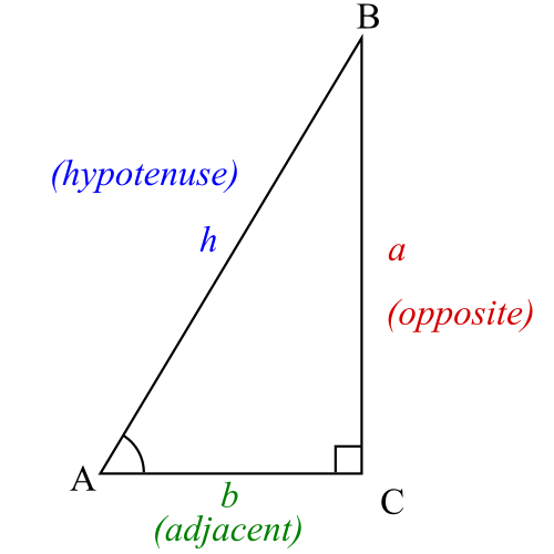
直角三角形の角度を求める 点の角度を基準とした辺を持つ 直角 三角形 。
A
{\displaystyle A}
逆三角関数は、直角 三角形の辺の長さがわかっている場合に、残りの2つの角度を決定するときに役立ちます 。直角三角形の正弦と余弦の定義を思い出すと、次のようになります。
θ
=
arcsin
(
opposite
hypotenuse
)
=
arccos
(
adjacent
hypotenuse
)
.
{\displaystyle \theta =\arcsin \left({\frac {\text{opposite}}{\text{hypotenuse}}}\right)=\arccos \left({\frac {\text{adjacent}}{\text{hypotenuse}}}\right).}
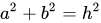
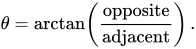
多くの場合、斜辺は不明であり、 ピタゴラスの定理を 使用してアークサインまたはアークコサインを使用する前に計算する必要があります。 ここで 、 は斜辺の長さです。この状況では、斜辺の長さは必要ないため、アークタンジェントが役立ちます。
a
2
+
b
2
=
h
2
{\displaystyle a^{2}+b^{2}=h^{2}}
h
{\displaystyle h}
θ
=
arctan
(
opposite
adjacent
)
.
{\displaystyle \theta =\arctan \left({\frac {\text{opposite}}{\text{adjacent}}}\right)\,.}
たとえば、屋根が 20 フィート伸びるときに 8 フィート下がるとします。屋根は 水平に対して θ の角度をなします。θ は 次のように計算できます。
θ
=
arctan
(
opposite
adjacent
)
=
arctan
(
rise
run
)
=
arctan
(
8
20
)
≈
21.8
∘
.
{\displaystyle \theta =\arctan \left({\frac {\text{opposite}}{\text{adjacent}}}\right)=\arctan \left({\frac {\text{rise}}{\text{run}}}\right)=\arctan \left({\frac {8}{20}}\right)\approx 21.8^{\circ }\,.}
コンピュータサイエンスとエンジニアリング
逆正接の2引数の変形
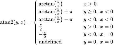
2 つの引数を取る atan2関数は、 y と x が与えられた場合に y / x の逆正接を計算します が、範囲は (− π 、 π ] です。言い換えると、 atan2( y 、 x ) は、平面の正の x軸とその上の点 ( x 、 y )の間の角度であり 、反時計回りの角度 (上半平面、 y > 0) の場合は正の符号、時計回りの角度 (下半平面、 y < 0) の場合は負の符号になります。これは、多くのコンピュータ プログラミング言語で最初に導入されましたが、現在では科学や工学の他の分野でも一般的になっています。
標準的な 逆正接 関数では、(− π / 2 、 π / 2 )、次のように表現できます。
atan2
(
y
,
x
)
=
{
arctan
(
y
x
)
x
>
0
arctan
(
y
x
)
+
π
y
≥
0
,
x
<
0
arctan
(
y
x
)
−
π
y
<
0
,
x
<
0
π
2
y
>
0
,
x
=
0
−
π
2
y
<
0
,
x
=
0
undefined
y
=
0
,
x
=
0
{\displaystyle \operatorname {atan2} (y,x)={\begin{cases}\arctan \left({\frac {y}{x}}\right)&\quad x>0\\\arctan \left({\frac {y}{x}}\right)+\pi &\quad y\geq 0,\;x<0\\\arctan \left({\frac {y}{x}}\right)-\pi &\quad y<0,\;x<0\\{\frac {\pi }{2}}&\quad y>0,\;x=0\\-{\frac {\pi }{2}}&\quad y<0,\;x=0\\{\text{undefined}}&\quad y=0,\;x=0\end{cases}}}
これは複素数 x + i y の 引数 の 主値 にも等しくなります 。
上記の関数のこの限定バージョンは、次のように 正接半角の公式 を使用して定義することもできます。
atan2
(
y
,
x
)
=
2
arctan
(
y
x
2
+
y
2
+
x
)
{\displaystyle \operatorname {atan2} (y,x)=2\arctan \left({\frac {y}{{\sqrt {x^{2}+y^{2}}}+x}}\right)}
ただし、 x > 0 または y ≠ 0の場合に限ります。 ただし、x ≤ 0 かつ y = 0 の場合は失敗するため、この式は計算には適していません。
上記の引数の順序 ( y 、 x ) は最も一般的であり、特に C プログラミング言語 などの ISO 標準で使用されていますが、少数の著者は逆の規則 ( x 、 y )を使用する可能性がある ため、注意が必要です。これらのバリエーションについては、 atan2 で詳しく説明されています。
位置パラメータ付き逆正接関数 多くの応用 [16] では、方程式の 解は 与えられた値に可能な限り近づくことである 。適切な解はパラメータ修正逆正接関数によって生成される。
y
{\displaystyle y}
x
=
tan
(
y
)
{\displaystyle x=\tan(y)}
−
∞
<
η
<
∞
{\displaystyle -\infty <\eta <\infty }
y
=
arctan
η
(
x
)
:=
arctan
(
x
)
+
π
rni
(
η
−
arctan
(
x
)
π
)
.
{\displaystyle y=\arctan _{\eta }(x):=\arctan(x)+\pi \,\operatorname {rni} \left({\frac {\eta -\arctan(x)}{\pi }}\right)\,.}
この関数は 最も近い整数に丸めます。
rni
{\displaystyle \operatorname {rni} }
数値精度 0 とπ に近い角度では アークコサインは 条件が悪く、 − π /2 と π /2に近い角度ではアークサインも同様に条件が悪く なります。したがって、コンピュータアプリケーションでは、これらの関数への入力の安定性と計算の感度を考慮するか、別の方法を使用する必要があります。 [17]
参照
注記
^ 「LHS RHS」という 表現は 、 (a) 左側 (つまり LHS) と右側 (つまり RHS) が 両方とも 真であるか、(b) 左側と右側が 両方とも 偽であることを示します。(c) という選択肢はありません ( つまり、 LHS ステートメントが真で、同時に RHS ステートメントが偽であるということはあり得ません)。そうでなければ、「LHS RHS 」は書かれなかったでしょう。
明確にするために、「LHS RHS」と書かれていて、LHS ( 左側 の 省略形 ) と RHS はどちらも個別に真または偽になり得るステートメントであるとします。たとえば、 と が 何らかの与えられた固定された数であり、次のように書かれるとします。LHS
はステートメント「 」です。 と が どのような特定の値を持つかによって 、この LHS ステートメントは真または偽になります。たとえば、 および の場合、LHS は真ですが ( この場合 であるため )、 および の場合、LHS は偽です (この場合 は と 等しくないため )。より一般的には、 および の場合には LHS は偽です 。 同様に、RHS は「 に対して」というステートメントです。RHS ステートメントも真または偽のいずれかになります (前述のように、RHS ステートメントが真か偽かは、 および がどのような特定の値を 持つかによって異なります)。論理等号記号 は、(a) LHS ステートメントが真であれば RHS ステートメントも 必然的に 真であり、さらに (b) LHS ステートメントが偽であれば RHS ステートメントも 必然的に 偽であることを意味します。同様に、 も (c) RHS ステートメントが真であれば LHS ステートメントも 必然的に 真であり、さらに (d) RHS ステートメントが偽であれば LHS ステートメントも 必然的に 偽であることを意味します。
⟺
{\displaystyle \,\iff \,}
⟺
{\displaystyle \,\iff \,}
⟺
{\displaystyle \,\iff \,}
θ
{\displaystyle \theta }
s
{\displaystyle s}
tan
θ
=
s
⟺
θ
=
arctan
(
s
)
+
π
k
for some
k
∈
Z
{\displaystyle \tan \theta =s\,\iff \,\theta =\arctan(s)+\pi k\quad {\text{ for some }}k\in \mathbb {Z} }
tan
θ
=
s
{\displaystyle \tan \theta =s}
θ
{\displaystyle \theta }
s
{\displaystyle s}
θ
=
0
{\displaystyle \theta =0}
s
=
0
{\displaystyle s=0}
tan
θ
=
tan
0
=
s
{\displaystyle \tan \theta =\tan 0=s}
θ
=
0
{\displaystyle \theta =0}
s
=
2
{\displaystyle s=2}
tan
θ
=
tan
0
=
s
{\displaystyle \tan \theta =\tan 0=s}
s
=
2
{\displaystyle s=2}
θ
=
0
{\displaystyle \theta =0}
s
≠
0.
{\displaystyle s\neq 0.}
θ
=
arctan
(
s
)
+
π
k
{\displaystyle \theta =\arctan(s)+\pi k}
k
∈
Z
{\displaystyle k\in \mathbb {Z} }
θ
{\displaystyle \theta }
s
{\displaystyle s}
⟺
{\displaystyle \,\iff \,}
⟺
{\displaystyle \,\iff \,}
参考文献
^ abcd Hall, Arthur Graham; Frink, Fred Goodrich (1909年1月). 「第2章 鋭角 [14] 逆三角関数」. 米国ミシガン州アナーバーで執筆。 三角法 。第1巻 パートI: 平面三角法。米国ニューヨーク: Henry Holt and Company / Norwood Press / JS Cushing Co. - Berwick & Smith Co.、米国マサチューセッツ州ノーウッド。p. 15。2017-08-12 に 取得 。 […] α = arcsin m : 2つの相互に逆の関数は、それぞれがもう一方の関数の反関数 であると言われるため、 「 アークサイン m 」または「 アンチサイン m 」とよく読みます 。 […] 同様の記号関係が他の 三角関数 にも当てはまります。 […] この表記法はヨーロッパで広く使用されており、米国でも急速に普及しています。あまり望ましくない記号 α = sin -1 m は 、英語やアメリカのテキストではまだ見られます。 α = inv sin m という表記は、 その一般的な適用性を考えると、おそらくさらに良いでしょう。 […] ^ クライン、フェリックス (1924) [1902]. Elementarmathematik vom höheren Standpunkt aus: 算術、代数、分析 (ドイツ語)。 Vol. 1 (第 3 版)。ベルリン:J.シュプリンガー。 高度な立場からの基礎数学:算術、代数、解析 として翻訳。ヘドリック、ER訳、ノーブル、CAマクミラン。1932年 。ISBN 978-0-486-43480-3 。 ^ Hazewinkel, Michiel (1994) [1987]. 数学百科事典 (完全版復刻版). Kluwer Academic Publishers / Springer Science & Business Media . ISBN 978-155608010-4 。
Bronshtein, IN; Semendyayev, KA; Musiol, Gerhard; Mühlig, Heiner. 「循環関数または逆三角関数」。 数学ハンドブック (第6版)。ベルリン:Springer。§ 2.8 、pp. 85–89。doi : 10.1007 /978-3-663-46221-8(2024年11月1日非アクティブ)。 {{cite book}}: CS1 maint: DOI inactive as of November 2024 (link)
ただし、「アーカス関数」という用語は、複素数の 引数を 与える関数を指す場合もあり、 アーカス と呼ばれることもあります。 ^ Weisstein, Eric W. 「逆三角関数」 。mathworld.wolfram.com 。 2020年8月29日 閲覧 。 ^ ビーチ、フレデリック・コンバース、ラインズ、ジョージ・エドウィン編 (1912)。「逆三角関数」。 アメリカーナ: ユニバーサル・リファレンス・ライブラリー 。第 21 巻。 ^ Cook, John D. (2021年2月11日). 「プログラミング言語間の三角関数」. johndcook.com (ブログ) . 2021年3月10日 閲覧 。 ^ カジョリ、フロリアン (1919年)。『数学の歴史』(第2版)。ニューヨーク、ニューヨーク: マクミラン社 。p.272。 ^ ハーシェル、ジョン・フレデリック・ウィリアム (1813年)。「コーツの定理の注目すべき応用について」。 哲学論文集 。103 (1)。王立協会、ロンドン:8。doi : 10.1098 / rstl.1813.0005 。 ^ 「逆三角関数」。Wiki。Brilliant Math & Science (brilliant.org) 。 2020年8月29日 閲覧 。 ^ Korn, Grandino Arthur; Korn, Theresa M. (2000) [1961]. 「21.2.-4. 逆三角関数」。科学者とエンジニアのための数学ハンドブック: 参照とレビュー の ための定義、定理、公式 (第 3 版)。ミネオラ、ニューヨーク、米国: Dover Publications、Inc . p. 811。ISBN 978-0-486-41147-7 。 ^ Bhatti, Sanaullah; Nawab-ud-Din; Ahmed, Bashir; Yousuf, SM; Taheem, Allah Bukhsh (1999)。「三角関数、対数関数、指数関数の微分」。Ellahi, Mohammad Maqbool; Dar, Karamat Hussain; Hussain, Faheem (編)。 微積分と解析幾何学 (第 1 版)。 ラホール : パンジャブ教科書委員会。p. 140。 ^ アブラモウィッツ&ステグン 1972、p.73、4.3.44 ^ ボルウェイン、ジョナサン、ベイリー、デイビッド、ジンガーソン、ローランド (2004)。数学における実験: 発見 への計算パス (第1版)。ウェルズリー、マサチューセッツ州、米国: AKピーターズ 。p.51。ISBN 978-1-56881-136-9 。 ^ Hwang Chien-Lih (2005)、「逆正接関数のオイラー級数の初等的導出」、 The Mathematical Gazette 、 89 (516): 469–470、 doi :10.1017/S0025557200178404、 S2CID 123395287 ^ SM Abrarov および BM Quine (2018)、「ネストされたラジカルを含む円周率の公式」、 The Ramanujan Journal 、 46 (3): 657–665、 arXiv : 1610.07713 、 doi :10.1007/s11139-018-9996-8、 S2CID 119150623 ^ 時間とともに変化する角度の交差を 鋸歯状の線ではなく滑らかな線で表すべき場合(ロボット工学、天文学、一般的な角度運動) [ 引用が必要 ]
±
π
/
2
{\displaystyle \pm \pi /2}
^ Gade, Kenneth (2010). 「非特異な水平位置表現」 (PDF) . The Journal of Navigation . 63 (3). Cambridge University Press : 395–417. Bibcode :2010JNav...63..395G. doi :10.1017/S0373463309990415.
外部リンク



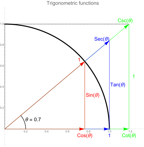


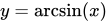








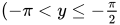

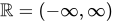




![{\displaystyle \mathbb {R} \setminus (-1,1)=(-\infty ,-1]\cup [1,\infty )}](https://wikimedia.org/api/rest_v1/media/math/render/svg/105fc2887189c9dbf0d165542a768dcd97f03069)


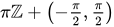















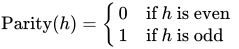




























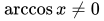















![{\displaystyle {\begin{aligned}\sin \theta &=-\sin(-\theta )&&=-\sin(\pi +\theta )&&={\phantom {-}}\sin(\pi -\theta )\\&=-\cos \left({\frac {\pi }{2}}+\theta \right)&&={\phantom {-}}\cos \left({\frac {\pi }{2}}-\theta \right)&&=-\cos \left(-{\frac {\pi }{2}}-\theta \right)\\&={\phantom {-}}\cos \left(-{\frac {\pi }{2}}+\theta \right)&&=-\cos \left({\frac {3\pi }{2}}-\theta \right)&&=-\cos \left(-{\frac {3\pi }{2}}+\theta \right)\\[0.3ex]\cos \theta &={\phantom {-}}\cos(-\theta )&&=-\cos(\pi +\theta )&&=-\cos(\pi -\theta )\\&={\phantom {-}}\sin \left({\frac {\pi }{2}}+\theta \right)&&={\phantom {-}}\sin \left({\frac {\pi }{2}}-\theta \right)&&=-\sin \left(-{\frac {\pi }{2}}-\theta \right)\\&=-\sin \left(-{\frac {\pi }{2}}+\theta \right)&&=-\sin \left({\frac {3\pi }{2}}-\theta \right)&&={\phantom {-}}\sin \left(-{\frac {3\pi }{2}}+\theta \right)\\[0.3ex]\tan \theta &=-\tan(-\theta )&&={\phantom {-}}\tan(\pi +\theta )&&=-\tan(\pi -\theta )\\&=-\cot \left({\frac {\pi }{2}}+\theta \right)&&={\phantom {-}}\cot \left({\frac {\pi }{2}}-\theta \right)&&={\phantom {-}}\cot \left(-{\frac {\pi }{2}}-\theta \right)\\&=-\cot \left(-{\frac {\pi }{2}}+\theta \right)&&={\phantom {-}}\cot \left({\frac {3\pi }{2}}-\theta \right)&&=-\cot \left(-{\frac {3\pi }{2}}+\theta \right)\\[0.3ex]\end{aligned}}}](https://wikimedia.org/api/rest_v1/media/math/render/svg/316baee0254e64a99779ac4721054f23295aeec6)




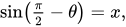











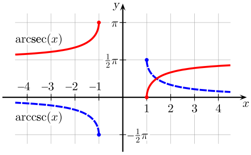
![{\displaystyle {\begin{aligned}\arccos(x)&={\frac {\pi }{2}}-\arcsin(x)\\[0.5em]\operatorname {arccot}(x)&={\frac {\pi }{2}}-\arctan(x)\\[0.5em]\operatorname {arccsc}(x)&={\frac {\pi }{2}}-\operatorname {arcsec}(x)\end{aligned}}}](https://wikimedia.org/api/rest_v1/media/math/render/svg/ec43798232f580abb074cf15f3d77692edd36af0)
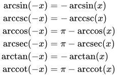
![{\displaystyle {\begin{aligned}\arcsin \left({\frac {1}{x}}\right)&=\operatorname {arccsc}(x)&\\[0.3em]\operatorname {arccsc} \left({\frac {1}{x}}\right)&=\arcsin(x)&\\[0.3em]\arccos \left({\frac {1}{x}}\right)&=\operatorname {arcsec}(x)&\\[0.3em]\operatorname {arcsec} \left({\frac {1}{x}}\right)&=\arccos(x)&\\[0.3em]\arctan \left({\frac {1}{x}}\right)&=\operatorname {arccot}(x)&={\frac {\pi }{2}}-\arctan(x)\,,{\text{ if }}x>0\\[0.3em]\arctan \left({\frac {1}{x}}\right)&=\operatorname {arccot}(x)-\pi &=-{\frac {\pi }{2}}-\arctan(x)\,,{\text{ if }}x<0\\[0.3em]\operatorname {arccot} \left({\frac {1}{x}}\right)&=\arctan(x)&={\frac {\pi }{2}}-\operatorname {arccot}(x)\,,{\text{ if }}x>0\\[0.3em]\operatorname {arccot} \left({\frac {1}{x}}\right)&=\arctan(x)+\pi &={\frac {3\pi }{2}}-\operatorname {arccot}(x)\,,{\text{ if }}x<0\end{aligned}}}](https://wikimedia.org/api/rest_v1/media/math/render/svg/a2fca7d530f42c84ed92b5895ccbafb013dc6645)


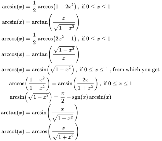


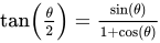
![{\displaystyle {\begin{aligned}\arcsin(x)&=2\arctan \left({\frac {x}{1+{\sqrt {1-x^{2}}}}}\right)\\[0.5em]\arccos(x)&=2\arctan \left({\frac {\sqrt {1-x^{2}}}{1+x}}\right)\,,{\text{ if }}-1<x\leq 1\\[0.5em]\arctan(x)&=2\arctan \left({\frac {x}{1+{\sqrt {1+x^{2}}}}}}\right)\end{aligned}}}](https://wikimedia.org/api/rest_v1/media/math/render/svg/7dd6a9370a877ca5e198e28b7582bd06b377bdc3)



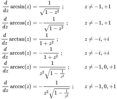
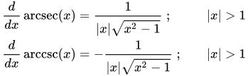



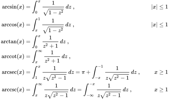


![{\displaystyle {\begin{aligned}\arcsin(z)&=z+\left({\frac {1}{2}}\right){\frac {z^{3}}{3}}+\left({\frac {1\cdot 3}{2\cdot 4}}\right){\frac {z^{5}}{5}}+\left({\frac {1\cdot 3\cdot 5}{2\cdot 4\cdot 6}}\right){\frac {z^{7}}{7}}+\cdots \\[5pt]&=\sum _{n=0}^{\infty }{\frac {(2n-1)!!}{(2n)!!}}{\frac {z^{2n+1}}{2n+1}}\\[5pt]&=\sum _{n=0}^{\infty }{\frac {(2n)!}{(2^{n}n!)^{2}}}{\frac {z^{2n+1}}{2n+1}}\,;\qquad |z|\leq 1\end{aligned}}}](https://wikimedia.org/api/rest_v1/media/math/render/svg/a0f778db7f760db059cf12f13ee5c2bf239fbb2f)



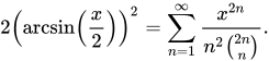




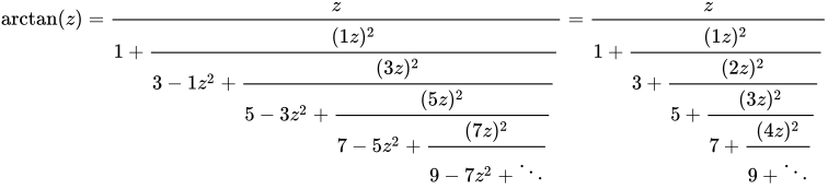
![{\displaystyle {\begin{aligned}\int \arcsin(z)\,dz&{}=z\,\arcsin(z)+{\sqrt {1-z^{2}}}+C\\\int \arccos(z)\,dz&{}=z\,\arccos(z)-{\sqrt {1-z^{2}}}+C\\\int \arctan(z)\,dz&{}=z\,\arctan(z)-{\frac {1}{2}}\ln \left(1+z^{2}\right)+C\\\int \operatorname {arccot}(z)\,dz&{}=z\,\operatorname {arccot}(z)+{\frac {1}{2}}\ln \left(1+z^{2}\right)+C\\\int \operatorname {arcsec}(z)\,dz&{}=z\,\operatorname {arcsec}(z)-\ln \left[z\left(1+{\sqrt {\frac {z^{2}-1}{z^{2}}}}\right)\right]+C\\\int \operatorname {arccsc}(z)\,dz&{}=z\,\operatorname {arccsc}(z)+\ln \left[z\left(1+{\sqrt {\frac {z^{2}-1}{z^{2}}}}\right)\right]+C\end{aligned}}}](https://wikimedia.org/api/rest_v1/media/math/render/svg/e3e2dde92bb82231c4326e45ce8b50e7298688bb)
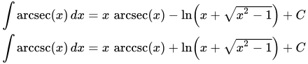

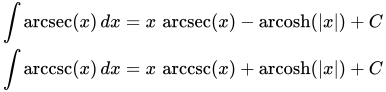
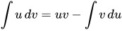
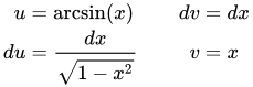










![{\displaystyle {\begin{aligned}\arcsin(z)&{}=-i\ln \left({\sqrt {1-z^{2}}}+iz\right)=i\ln \left({\sqrt {1-z^{2}}}-iz\right)&{}=\operatorname {arccsc} \left({\frac {1}{z}}\right)\\[10pt]\arccos(z)&{}=-i\ln \left(i{\sqrt {1-z^{2}}}+z\right)={\frac {\pi }{2}}-\arcsin(z)&{}=\operatorname {arcsec} \left({\frac {1}{z}}\right)\\[10pt]\arctan(z)&{}=-{\frac {i}{2}}\ln \left({\frac {iz}{i+z}}\right)=-{\frac {i}{2}}\ln \left({\frac {1+iz}{1-iz}}\right)&{}=\operatorname {arccot} \left({\frac {1}{z}}\right)\\[10pt]\operatorname {arccot}(z)&{}=-{\frac {i}{2}}\ln \left({\frac {z+i}{zi}}\right)=-{\frac {i}{2}}\ln \left({\frac {iz-1}{iz+1}}\right)&{}=\arctan \left({\frac {1}{z}}\right)\\[10pt]\operatorname {arcsec}(z)&{}=-i\ln \left(i{\sqrt {1-{\frac {1}{z^{2}}}}}+{\frac {1}{z}}\right)={\frac {\pi }{2}}-\operatorname {arccsc}(z)&{}=\arccos \left({\frac {1}{z}}\right)\\[10pt]\operatorname {arccsc}(z)&{}=-i\ln \left({\sqrt {1-{\frac {1}{z^{2}}}}}+{\frac {i}{z}}\right)=i\ln \left({\sqrt {1-{\frac {1}{z^{2}}}}}-{\frac {i}{z}}\right)&{}=\arcsin \left({\frac {1}{z}}\right)\end{aligned}}}](https://wikimedia.org/api/rest_v1/media/math/render/svg/13b511be341b52fcd0c0660f3a4b1e5a164bfcb1)

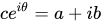


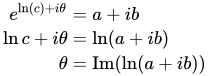
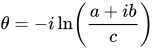


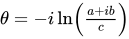

![{\displaystyle \operatorname {Im} \left(\ln z\right)\in (-\pi ,\pi ]}](https://wikimedia.org/api/rest_v1/media/math/render/svg/781cef7f2317c18794eeaaddeef4073aadd51b75)



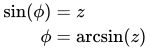

![{\displaystyle {\begin{aligned}z&={\frac {e^{i\phi }-e^{-i\phi }}{2i}}\\[10mu]2iz&=\xi -{\frac { 1}{\xi }}\\[5mu]0&=\xi ^{2}-2iz\xi -1\\[5mu]\xi &=iz\pm {\sqrt {1-z^{2}}}\\[5mu]\phi &=-i\ln \left(iz\pm {\sqrt {1-z^{2}}}\right)\end{aligned} }}](https://wikimedia.org/api/rest_v1/media/math/render/svg/ed03e8cf773fa44cc78823d65f7d82f41276fb96)