例
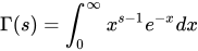
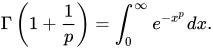
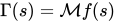
指数関数 について p > 0 {\displaystyle p>0} て f ( x ) = e − p x {\displaystyle f(x)=e^{-px}} M f ( s ) = ∫ 0 ∞ x s e − p x d x x = ∫ 0 ∞ ( u p ) s e − u d u u = 1 p s ∫ 0 ∞ u s e − u d u u = 1 p s Γ ( s ) 。 {\displaystyle {\mathcal {M}}f(s)=\int _{0}^{\infty }x^{s}e^{-px}{\frac {dx}{x}}=\int _{0}^{\infty }\left({\frac {u}{p}}\right)^{s}e^{-u}{\frac {du}{u}}={\frac {1}{p^{s}}}\int _{0}^{\infty }u^{s}e^{-u}{\frac {du}{u}}={\frac {1}{p^{s}}}\Gamma (s).}
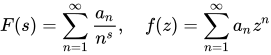
冪級数とディリクレ級数 一般的に、必要な収束を仮定すると、ディリクレ級数と冪級数を関連付けることができる。 F ( s ) = ∑ n = 1 ∞ 1 n n s 、 f ( z ) = ∑ n = 1 ∞ 1 n z n {\displaystyle F(s)=\sum \limits _{n=1}^{\infty }{\frac {a_{n}}{n^{s}}},\quad f(z)=\sum \limits _{n=1}^{\infty }a_{n}z^{n}} [ 5 ] Γ ( s ) F ( s ) = ∫ 0 ∞ x s − 1 f ( e − x ) d x {\displaystyle \Gamma (s)F(s)=\int _{0}^{\infty }x^{s-1}f(e^{-x})dx}
物件 この表に記載されている特性は、Bracewell (2000) およびErdélyi (1954) に記載されています。
させてf 1 ( x ) {\displaystyle f_{1}(x)} f 2 ( x ) {\displaystyle f_{2}(x)} f ~ 1 、 2 ( s ) = M { f 1 、 2 } ( s ) {\displaystyle {\tilde {f}}_{1,2}(s)={\mathcal {M}}\{f_{1,2}\}(s)} 基本 α 1 、 2 < ℜ s < β 1 、 2 {\displaystyle \alpha _{1,2}<\Re s<\beta _{1,2}} c ∈ R {\displaystyle c\in \mathbb {R} } 最大 ( α 1 、 1 − β 2 ) < c < ミニ ( β 1 、 1 − α 2 ) {\displaystyle \max(\alpha _{1},1-\beta _{2})<c<\min(\beta _{1},1-\alpha _{2})} x c − 1 / 2 f 1 ( x ) {\displaystyle x^{c-1/2}\,f_{1}(x)} x 1 / 2 − c f 2 ( x ) {\displaystyle x^{1/2-c}\,f_{2}(x)} 。 ( 0 、 ∞ ) {\displaystyle (0,\infty )} パーセバルの公式 が成り立つ: [ 7 ] ∫ 0 ∞ f 1 ( x ) f 2 ( x ) d x = 1 2 π 私 ∫ c − 私 ∞ c + 私 ∞ f 1 ~ ( s ) f 2 ~ ( 1 − s ) d s {\displaystyle \int _{0}^{\infty }f_{1}(x)\,f_{2}(x)\,dx={\frac {1}{2\pi i}}\int _{c-i\infty }^{c+i\infty }{\tilde {f_{1}}}(s)\,{\tilde {f_{2}}}(1-s)\,ds} ℜ r = c {\displaystyle \Re r=c}
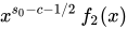
交換できますf 2 ( x ) {\displaystyle f_{2}(x)} よる f 2 ( x ) x s 0 − 1 {\displaystyle f_{2}(x)\,x^{s_{0}-1}} f 1 ( x ) {\displaystyle f_{1}(x)} f 2 ( x ) {\displaystyle f_{2}(x)} f ~ 1 、 2 ( s ) = M { f 1 、 2 } ( s ) {\displaystyle {\tilde {f}}_{1,2}(s)={\mathcal {M}}\{f_{1,2}\}(s)} 基本 α 1 、 2 < ℜ s < β 1 、 2 {\displaystyle \alpha _{1,2}<\Re s<\beta _{1,2}} c ∈ R {\displaystyle c\in \mathbb {R} } α 1 < c < β 1 {\displaystyle \alpha _{1}<c<\beta _{1}} s 0 ∈ C {\displaystyle s_{0}\in \mathbb {C} } α 2 < ℜ s 0 − c < β 2 {\displaystyle \alpha _{2}<\Re s_{0}-c<\beta _{2}} x c − 1 / 2 f 1 ( x ) {\displaystyle x^{c-1/2}\,f_{1}(x)} x s 0 − c − 1 / 2 f 2 ( x ) {\displaystyle x^{s_{0}-c-1/2}\,f_{2}(x)} ( 0 、 ∞ ) {\displaystyle (0,\infty )} [ 7 ] ∫ 0 ∞ f 1 ( x ) f 2 ( x ) x s 0 − 1 d x = 1 2 π 私 ∫ c − 私 ∞ c + 私 ∞ f 1 ~ ( s ) f 2 ~ ( s 0 − s ) d s {\displaystyle \int _{0}^{\infty }f_{1}(x)\,f_{2}(x)\,x^{s_{0}-1}\,dx={\frac {1}{2\pi i}}\int _{c-i\infty }^{c+i\infty }{\tilde {f_{1}}}(s)\,{\tilde {f_{2}}}(s_{0}-s)\,ds} f 2 ( x ) {\displaystyle f_{2}(x)} よる f 1 ( x ) ¯ {\displaystyle {\overline {f_{1}(x)}}} f ( x ) {\displaystyle f(x)} f ~ ( s ) = M { f } ( s ) {\displaystyle {\tilde {f}}(s)={\mathcal {M}}\{f\}(s)} において α < ℜ s < β {\displaystyle \alpha <\Re s<\beta } c ∈ R {\displaystyle c\in \mathbb {R} } α < c < β {\displaystyle \alpha <c<\beta } x c − 1 / 2 f ( x ) {\displaystyle x^{c-1/2}\,f(x)} 。 ( 0 、 ∞ ) {\displaystyle (0,\infty )} プランシュレルの定理 が成り立つ: [ 8 ] ∫ 0 ∞ | f ( x ) | 2 x 2 c − 1 d x = 1 2 π ∫ − ∞ ∞ | f ~ ( c + 私 t ) | 2 d t {\displaystyle \int _{0}^{\infty }|f(x)|^{2}\,x^{2c-1}dx={\frac {1}{2\pi }}\int _{-\infty }^{\infty }|{\tilde {f}}(c+it)|^{2}\,dt}
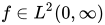
L2 空間上の 等長変換としてヒルベルト空間 の研究では、メリン変換はしばしば少し異なる形で定式化される。L 2 ( 0 、 ∞ ) {\displaystyle L^{2}(0,\infty )} L p 1 2 + 私 R {\displaystyle {\tfrac {1}{2}}+i\mathbb {R} } 線形演算子を定義することができます M ~ {\displaystyle {\tilde {\mathcal {M}}}} M ~ : L 2 ( 0 、 ∞ ) → L 2 ( − ∞ 、 ∞ ) 、 {\displaystyle {\tilde {\mathcal {M}}}\colon L^{2}(0,\infty )\to L^{2}(-\infty ,\infty ),} { M ~ f } ( s ) := 1 2 π ∫ 0 ∞ x − 1 2 + 私 s f ( x ) d x 。 {\displaystyle \{{\tilde {\mathcal {M}}}f\}(s):={\frac {1}{\sqrt {2\pi }}}\int _{0}^{\infty }x^{-{\frac {1}{2}}+is}f(x)\,dx.} { M ~ f } ( s ) := 1 2 π { M f } ( 1 2 + 私 s ) 。 {\displaystyle \{{\tilde {\mathcal {M}}}f\}(s):={\tfrac {1}{\sqrt {2\pi }}}\{{\mathcal {M}}f\}({\tfrac {1}{2}}+is).} M {\displaystyle {\mathcal {M}}} M ~ {\displaystyle {\tilde {\mathcal {M}}}} メリン反転定理は 、次のことを示している。M ~ {\displaystyle {\tilde {\mathcal {M}}}} M ~ − 1 : L 2 ( − ∞ 、 ∞ ) → L 2 ( 0 、 ∞ ) 、 {\displaystyle {\tilde {\mathcal {M}}}^{-1}\colon L^{2}(-\infty ,\infty )\to L^{2}(0,\infty ),} { M ~ − 1 φ } ( x ) = 1 2 π ∫ − ∞ ∞ x − 1 2 − 私 s φ ( s ) d s 。 {\displaystyle \{{\tilde {\mathcal {M}}}^{-1}\varphi \}(x)={\frac {1}{\sqrt {2\pi }}}\int _{-\infty }^{\infty }x^{-{\frac {1}{2}}-is}\varphi (s)\,ds.} 等長変換 である。つまり、‖ M ~ f ‖ L 2 ( − ∞ 、 ∞ ) = ‖ f ‖ L 2 ( 0 、 ∞ ) {\displaystyle \|{\tilde {\mathcal {M}}}f\|_{L^{2}(-\infty ,\infty )}=\|f\|_{L^{2}(0,\infty )}} f ∈ L 2 ( 0 、 ∞ ) {\displaystyle f\in L^{2}(0,\infty )} 1 / 2 π {\displaystyle 1/{\sqrt {2\pi }}}
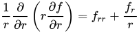
円筒座標系におけるラプラシアンの問題点 一般的な次元( 1つの角度と1つの半径、および残りの長さを持つ 直交座標 )における円筒座標のラプラシアンには、常に次の項があります。1 r ∂ ∂ r ( r ∂ f ∂ r ) = f r r + f r r {\displaystyle {\frac {1}{r}}{\frac {\partial }{\partial r}}\left(r{\frac {\partial f}{\partial r}}\right)=f_{rr}+{\frac {f_{r}}{r}}}
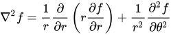
例えば、2次元極座標におけるラプラシアンは次のようになります。 ∇ 2 f = 1 r ∂ ∂ r ( r ∂ f ∂ r ) + 1 r 2 ∂ 2 f ∂ θ 2 {\displaystyle \nabla ^{2}f={\frac {1}{r}}{\frac {\partial }{\partial r}}\left(r{\frac {\partial f}{\partial r}}\right)+{\frac {1}{r^{2}}}{\frac {\partial ^{2}f}{\partial \theta ^{2}}}} ∇ 2 f = 1 r ∂ ∂ r ( r ∂ f ∂ r ) + 1 r 2 ∂ 2 f ∂ φ 2 + ∂ 2 f ∂ z 2 。 {\displaystyle \nabla ^{2}f={\frac {1}{r}}{\frac {\partial }{\partial r}}\left(r{\frac {\partial f}{\partial r}}\right)+{\frac {1}{r^{2}}}{\frac {\partial ^{2}f}{\partial \varphi ^{2}}}+{\frac {\partial ^{2}f}{\partial z^{2}}}.}
この項は、メリン変換[ 12 ] M ( r 2 f r r + r f r 、 r → s ) = s 2 M ( f 、 r → s ) = s 2 F {\displaystyle {\mathcal {M}}\left(r^{2}f_{rr}+rf_{r},r\to s\right)=s^{2}{\mathcal {M}}\left(f,r\to s\right)=s^{2}F}
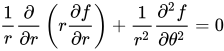
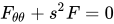
例えば、極座標における 2次元ラプラス方程式は、2変数偏微分方程式で表されます。 r 2 f r r + r f r + f θ θ = 0 {\displaystyle r^{2}f_{rr}+rf_{r}+f_{\theta \theta }=0} 1 r ∂ ∂ r ( r ∂ f ∂ r ) + 1 r 2 ∂ 2 f ∂ θ 2 = 0 {\displaystyle {\frac {1}{r}}{\frac {\partial }{\partial r}}\left(r{\frac {\partial f}{\partial r}}\right)+{\frac {1}{r^{2}}}{\frac {\partial ^{2}f}{\partial \theta ^{2}}}=0} 調和振動子 となる。 F θ θ + s 2 F = 0 {\displaystyle F_{\theta \theta }+s^{2}F=0} F ( s 、 θ ) = C 1 ( s ) コス ( s θ ) + C 2 ( s ) 罪 ( s θ ) {\displaystyle F(s,\theta )=C_{1}(s)\cos(s\theta )+C_{2}(s)\sin(s\theta )}
それでは、例えば、元のラプラス方程式に いくつかの単純なくさび境界条件を課してみましょう。 f ( r 、 − θ 0 ) = 1 ( r ) 、 f ( r 、 θ 0 ) = b ( r ) {\displaystyle f(r,-\theta _{0})=a(r),\quad f(r,\theta _{0})=b(r)} F ( s 、 − θ 0 ) = A ( s ) 、 F ( s 、 θ 0 ) = B ( s ) {\displaystyle F(s,-\theta _{0})=A(s),\quad F(s,\theta _{0})=B(s)}
これらの条件を解に課すことで、解は以下のように具体化される。 F ( s 、 θ ) = A ( s ) 罪 ( s ( θ 0 − θ ) ) 罪 ( 2 θ 0 s ) + B ( s ) 罪 ( s ( θ 0 + θ ) ) 罪 ( 2 θ 0 s ) {\displaystyle F(s,\theta )=A(s){\frac {\sin(s(\theta _{0}-\theta ))}{\sin(2\theta _{0}s)}}+B(s){\frac {\sin(s(\theta _{0}+\theta ))}{\sin(2\theta _{0}s)}}}
メリン変換の畳み込み定理により、メリン領域における解は逆変換できる。 f ( r 、 θ ) = r m コス ( m θ ) 2 θ 0 ∫ 0 ∞ ( 1 ( x ) x 2 m + 2 r m x m 罪 ( m θ ) + r 2 m + b ( x ) x 2 m − 2 r m x m 罪 ( m θ ) + r 2 m ) x m − 1 d x {\displaystyle f(r,\theta )={\frac {r^{m}\cos(m\theta )}{2\theta _{0}}}\int _{0}^{\infty }\left({\frac {a(x)}{x^{2m}+2r^{m}x^{m}\sin(m\theta )+r^{2m}}}+{\frac {b(x)}{x^{2m}-2r^{m}x^{m}\sin(m\theta )+r^{2m}}}\right)x^{m-1}\,dx} M − 1 ( 罪 ( s φ ) 罪 ( 2 θ 0 s ) ; s → r ) = 1 2 θ 0 r m 罪 ( m φ ) 1 + 2 r m コス ( m φ ) + r 2 m {\displaystyle {\mathcal {M}}^{-1}\left({\frac {\sin(s\varphi )}{\sin(2\theta _{0}s)}};s\to r\right)={\frac {1}{2\theta _{0}}}{\frac {r^{m}\sin(m\varphi )}{1+2r^{m}\cos(m\varphi )+r^{2m}}}} m = π 2 θ 0 {\displaystyle m={\frac {\pi }{2\theta _{0}}}}
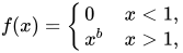
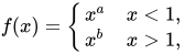
以下に、メリン変換の興味深い例をいくつか示します。
注記 ↑ メリン、Hj. 「Zur Theorie zweier allgemeinen Klassen bestimmter Integrale」。Acta Societatis Scientiarum Fennicae 。XXII (2): 1-75 . ↑ Whittaker, ET ; Watson, GN (1996). A Course of Modern Analysis . Cambridge University Press. ↑ Hardy, GH ; Littlewood, JE (1916). "Contributions to the Theory of the Riemann Zeta-Function and the Theory of the Distribution of Primes" . Acta Mathematica . 41 (1): 119– 196. doi : 10.1007/BF02422942 . カヘンとメリンの著作、およびカヘンの論文に関する詳細な参考文献については、同書中の注釈を参照のこと。 )↑ Wintner, Aurel (1947). "On Riemann's Reduction of Dirichlet Series to Power Series" . American Journal of Mathematics . 69 (4): 769–789 . doi : 10.2307/2371798 . JSTOR 2371798 . 1 2 ティッチマーシュ(1948年 、95ページ ) 。 ↑ ティッチマーシュ (1948 、p. 94) 。 ↑ ガランボス& シモネリ (2004 、p. 15) 1 2 3 ガランボス& シモネリ (2004 、p. 16) ↑ ガランボス& シモネリ (2004 、p. 23) ↑ Bhimsen、Shivamoggi、第6章:メリン変換、第4.3節:ウェッジ内のポテンシャルの分布、267~268ページ ↑ フィリップ・フラジョレとロバート・セジウィック。アルゴリズムの平均ケース分析: メリン変換漸近線。研究報告書 2956、93 ページ。国立情報学・自動車技術研究所 (INRIA)、1996 年。 ↑ A. リアム・フィッツパトリック、ジャレッド・カプラン、ジョアン・ペネドネス、スブラト・ラジュ、バルト・C・ヴァン・リース。「AdS/CFT相関関係者のための自然言語」。 ↑ A. リアム・フィッツパトリック、ジャレッド・カプラン。「ユニタリティとホログラフィックSマトリックス」 ↑ A. リアム・フィッツパトリック。 「AdS/CFTとホログラフィックSマトリックス」、ビデオ講義。 ↑ ベルトラン、ジャクリーン;ベルトラン、ピエール;オヴァルレ、ジャン=フィリップ(1995)。 『メリン変換:変換と応用ハンドブック 』テイラー&フランシス 。ISBN 978-1420066524 。
参考文献 ブレイスウェル、ロナルド N. (2000).フーリエ変換とその応用 (第 3 版) デブナス、ロケナス。バッタ、ダンバルー(2016 年 4 月 19 日)。積分変換とその応用 。 CRCプレス。ISBN 978-1-4200-1091-6 。 エプスタイン、ベンジャミン。「統計学におけるメリン変換のいくつかの応用」。カーネギーメロン工科大学。 エルデリー、アーサー(1954)。積分変換表 。第 1巻。マグロウヒル。 Flajolet, P.; Gourdon, X.; Dumas, P. (1995). "Mellin変換と漸近解析:調和和" (PDF) . Theoretical Computer Science . 144 ( 1– 2): 3– 58. doi : 10.1016/0304-3975(95)00002-e . Galambos, Janos; Simonelli, Italo (2004).確率変数の積:物理学の問題と算術関数への応用 ISBN 0-8247-5402-6 。 Paris, RB; Kaminski, D. (2001).漸近解析とメリン・バーンズ積分 ISBN 9780521790017 。 ポリャニン、AD; マンジロフ、AV (1998).積分方程式ハンドブック . フロリダ州ボカラトン: CRC Press. ISBN 0-8493-2876-4 。 ティッチマーシュ、EC(1948)。フーリエ積分理論入門 (第2 版)。 ポリャニン、アンドレイ D. 「積分変換の表」。EqWorld : 数学方程式の世界 。 「メリン変換」、数学百科事典 EMS Press 、2001 [1994] Weisstein, Eric W. 「メリン変換」 . MathWorld
外部リンク Philippe Flajolet、Xavier Gourdon、Philippe Dumas、「メリン変換と漸近解析:調和和」 アントニオ ゴンザレス、マルコ リーデル クラシコのセレブランド、ニュースグループ es.ciencia.matematicas フアン・サセルドティ、ファンシオネス・エウレリアナス (スペイン語)。 メリン変換法、数学関数デジタルライブラリ 、2011年8月29日、米国国立標準技術研究所 アントニオ・デ・セナとダヴィデ・ロッケッソ、「DAFXへの応用を伴う高速メリン変換」