数学的恒等式
以下は ベクトル解析 における微分と積分に関する重要な 恒等式 です。
演算子表記
勾配 3次元 直交座標 変数の関数の場合 、勾配はベクトル場です。
f
(
x
,
y
,
z
)
{\displaystyle f(x,y,z)}
grad
(
f
)
=
∇
f
=
(
∂
∂
x
,
∂
∂
y
,
∂
∂
z
)
f
=
∂
f
∂
x
i
+
∂
f
∂
y
j
+
∂
f
∂
z
k
{\displaystyle \operatorname {grad} (f)=\nabla f={\begin{pmatrix}\displaystyle {\frac {\partial }{\partial x}},\ {\frac {\partial }{\partial y}},\ {\frac {\partial }{\partial z}}\end{pmatrix}}f={\frac {\partial f}{\partial x}}\mathbf {i} +{\frac {\partial f}{\partial y}}\mathbf {j} +{\frac {\partial f}{\partial z}}\mathbf {k} }
ここで、 i 、 j 、 kは x 、 y 、 z 軸の 標準 単位ベクトル です。より一般的には、 スカラー 場とも呼ばれる n 変数 の関数の場合 、勾配は ベクトル場 です。
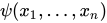
ここで、 は互いに直交する単位ベクトルです。
ψ
(
x
1
,
…
,
x
n
)
{\displaystyle \psi (x_{1},\ldots ,x_{n})}
∇
ψ
=
(
∂
∂
x
1
,
…
,
∂
∂
x
n
)
ψ
=
∂
ψ
∂
x
1
e
1
+
⋯
+
∂
ψ
∂
x
n
e
n
{\displaystyle \nabla \psi ={\begin{pmatrix}\displaystyle {\frac {\partial }{\partial x_{1}}},\ldots ,{\frac {\partial }{\partial x_{n}}}\end{pmatrix}}\psi ={\frac {\partial \psi }{\partial x_{1}}}\mathbf {e} _{1}+\dots +{\frac {\partial \psi }{\partial x_{n}}}\mathbf {e} _{n}}
e
i
(
i
=
1
,
2
,
.
.
.
,
n
)
{\displaystyle \mathbf {e} _{i}\,(i=1,2,...,n)}
名前が示すように、勾配は関数の最も急速な (正の) 変化に比例し、その方向を指します。
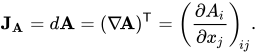
ベクトル場( 1次のテンソル場とも呼ばれる)の場合、勾配または 全微分は n×nの ヤコビ行列 である 。
A
=
(
A
1
,
…
,
A
n
)
{\displaystyle \mathbf {A} =\left(A_{1},\ldots ,A_{n}\right)}
J
A
=
d
A
=
(
∇
A
)
T
=
(
∂
A
i
∂
x
j
)
i
j
.
{\displaystyle \mathbf {J} _{\mathbf {A} }=d\mathbf {A} =(\nabla \!\mathbf {A} )^{\textsf {T}}=\left({\frac {\partial A_{i}}{\partial x_{j}}}\right)_{\!ij}.}
任意の次数 kの テンソル場 の場合 、勾配は次数 k + 1のテンソル場です 。
T
{\displaystyle \mathbf {T} }
grad
(
T
)
=
d
T
=
(
∇
T
)
T
{\displaystyle \operatorname {grad} (\mathbf {T} )=d\mathbf {T} =(\nabla \mathbf {T} )^{\textsf {T}}}
k > 0の テンソル場の場合、 k + 1の テンソル場は、任意の定数ベクトル
である 再帰関係によって定義されます
。
T
{\displaystyle \mathbf {T} }
∇
T
{\displaystyle \nabla \mathbf {T} }
(
∇
T
)
⋅
C
=
∇
(
T
⋅
C
)
{\displaystyle (\nabla \mathbf {T} )\cdot \mathbf {C} =\nabla (\mathbf {T} \cdot \mathbf {C} )}
C
{\displaystyle \mathbf {C} }
発散 デカルト座標では、連続的に微分可能な ベクトル場 の発散は スカラー値関数です。
F
=
F
x
i
+
F
y
j
+
F
z
k
{\displaystyle \mathbf {F} =F_{x}\mathbf {i} +F_{y}\mathbf {j} +F_{z}\mathbf {k} }
div
F
=
∇
⋅
F
=
(
∂
∂
x
,
∂
∂
y
,
∂
∂
z
)
⋅
(
F
x
,
F
y
,
F
z
)
=
∂
F
x
∂
x
+
∂
F
y
∂
y
+
∂
F
z
∂
z
.
{\displaystyle \operatorname {div} \mathbf {F} =\nabla \cdot \mathbf {F} ={\begin{pmatrix}\displaystyle {\frac {\partial }{\partial x}},\ {\frac {\partial }{\partial y}},\ {\frac {\partial }{\partial z}}\end{pmatrix}}\cdot {\begin{pmatrix}F_{x},\ F_{y},\ F_{z}\end{pmatrix}}={\frac {\partial F_{x}}{\partial x}}+{\frac {\partial F_{y}}{\partial y}}+{\frac {\partial F_{z}}{\partial z}}.}
名前が示すように、発散は、フィールド内のベクトルが発散する度合いの (ローカルな) 尺度です。
非ゼロ次 kの テンソル場 の発散は 、次数 k − 1のテンソル場の 縮約 として表されます 。具体的には、ベクトルの発散はスカラーです。より高次のテンソル場の発散は、テンソル場を外積の和に分解し 、 恒等式を使用すること
で求められます。
ここで、は の方向の 方向 微分にその大きさを乗じたもの です 。具体的には、2 つのベクトルの外積の場合、
T
{\displaystyle \mathbf {T} }
div
(
T
)
=
∇
⋅
T
{\displaystyle \operatorname {div} (\mathbf {T} )=\nabla \cdot \mathbf {T} }
∇
⋅
(
A
⊗
T
)
=
T
(
∇
⋅
A
)
+
(
A
⋅
∇
)
T
{\displaystyle \nabla \cdot \left(\mathbf {A} \otimes \mathbf {T} \right)=\mathbf {T} (\nabla \cdot \mathbf {A} )+(\mathbf {A} \cdot \nabla )\mathbf {T} }
A
⋅
∇
{\displaystyle \mathbf {A} \cdot \nabla }
A
{\displaystyle \mathbf {A} }
∇
⋅
(
A
B
T
)
=
B
(
∇
⋅
A
)
+
(
A
⋅
∇
)
B
.
{\displaystyle \nabla \cdot \left(\mathbf {A} \mathbf {B} ^{\textsf {T}}\right)=\mathbf {B} (\nabla \cdot \mathbf {A} )+(\mathbf {A} \cdot \nabla )\mathbf {B} .}
k > 1の テンソル場に対して、 k − 1の テンソル場は、 任意の定数ベクトル
である 再帰関係によって定義されます
。
T
{\displaystyle \mathbf {T} }
∇
⋅
T
{\displaystyle \nabla \cdot \mathbf {T} }
(
∇
⋅
T
)
⋅
C
=
∇
⋅
(
T
⋅
C
)
{\displaystyle (\nabla \cdot \mathbf {T} )\cdot \mathbf {C} =\nabla \cdot (\mathbf {T} \cdot \mathbf {C} )}
C
{\displaystyle \mathbf {C} }
カール デカルト座標では、 回転はベクトル場です。
ここで、 i 、 j 、 kはそれぞれ x 軸、 y 軸、 z 軸の 単位ベクトル です 。
F
=
F
x
i
+
F
y
j
+
F
z
k
{\displaystyle \mathbf {F} =F_{x}\mathbf {i} +F_{y}\mathbf {j} +F_{z}\mathbf {k} }
curl
F
=
∇
×
F
=
(
∂
∂
x
,
∂
∂
y
,
∂
∂
z
)
×
(
F
x
,
F
y
,
F
z
)
=
|
i
j
k
∂
∂
x
∂
∂
y
∂
∂
z
F
x
F
y
F
z
|
=
(
∂
F
z
∂
y
−
∂
F
y
∂
z
)
i
+
(
∂
F
x
∂
z
−
∂
F
z
∂
x
)
j
+
(
∂
F
y
∂
x
−
∂
F
x
∂
y
)
k
{\displaystyle {\begin{aligned}\operatorname {curl} \mathbf {F} &=\nabla \times \mathbf {F} ={\begin{pmatrix}\displaystyle {\frac {\partial }{\partial x}},\ {\frac {\partial }{\partial y}},\ {\frac {\partial }{\partial z}}\end{pmatrix}}\times {\begin{pmatrix}F_{x},\ F_{y},\ F_{z}\end{pmatrix}}={\begin{vmatrix}\mathbf {i} &\mathbf {j} &\mathbf {k} \\{\frac {\partial }{\partial x}}&{\frac {\partial }{\partial y}}&{\frac {\partial }{\partial z}}\\F_{x}&F_{y}&F_{z}\end{vmatrix}}\\[1em]&=\left({\frac {\partial F_{z}}{\partial y}}-{\frac {\partial F_{y}}{\partial z}}\right)\mathbf {i} +\left({\frac {\partial F_{x}}{\partial z}}-{\frac {\partial F_{z}}{\partial x}}\right)\mathbf {j} +\left({\frac {\partial F_{y}}{\partial x}}-{\frac {\partial F_{x}}{\partial y}}\right)\mathbf {k} \end{aligned}}}
名前が示すように、回転は、近くのベクトルが円形の方向にどれだけ傾向があるかを測定するものです。
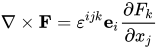
アインシュタイン表記 では 、ベクトル場の 回転は次のように表されます。
ここで、 = ±1 または 0 は レヴィ-チヴィタ パリティ記号 です。
F
=
(
F
1
,
F
2
,
F
3
)
{\displaystyle \mathbf {F} ={\begin{pmatrix}F_{1},\ F_{2},\ F_{3}\end{pmatrix}}}
∇
×
F
=
ε
i
j
k
e
i
∂
F
k
∂
x
j
{\displaystyle \nabla \times \mathbf {F} =\varepsilon ^{ijk}\mathbf {e} _{i}{\frac {\partial F_{k}}{\partial x_{j}}}}
ε
{\displaystyle \varepsilon }
k > 1 の位数の テンソル場の場合、 k の位数の テンソル場は、任意の定数ベクトル
である 再帰関係によって定義されます
。
T
{\displaystyle \mathbf {T} }
∇
×
T
{\displaystyle \nabla \times \mathbf {T} }
(
∇
×
T
)
⋅
C
=
∇
×
(
T
⋅
C
)
{\displaystyle (\nabla \times \mathbf {T} )\cdot \mathbf {C} =\nabla \times (\mathbf {T} \cdot \mathbf {C} )}
C
{\displaystyle \mathbf {C} }
1より大きい位数のテンソル体は 外積 の和に分解することができ、次の恒等式を使用することができる。
具体的には、2つのベクトルの外積については、
∇
×
(
A
⊗
T
)
=
(
∇
×
A
)
⊗
T
−
A
×
(
∇
T
)
.
{\displaystyle \nabla \times \left(\mathbf {A} \otimes \mathbf {T} \right)=(\nabla \times \mathbf {A} )\otimes \mathbf {T} -\mathbf {A} \times (\nabla \mathbf {T} ).}
∇
×
(
A
B
T
)
=
(
∇
×
A
)
B
T
−
A
×
(
∇
B
)
.
{\displaystyle \nabla \times \left(\mathbf {A} \mathbf {B} ^{\textsf {T}}\right)=(\nabla \times \mathbf {A} )\mathbf {B} ^{\textsf {T}}-\mathbf {A} \times (\nabla \mathbf {B} ).}
ラプラシアン 直交座標 では 、関数のラプラシアン は
f
(
x
,
y
,
z
)
{\displaystyle f(x,y,z)}
Δ
f
=
∇
2
f
=
(
∇
⋅
∇
)
f
=
∂
2
f
∂
x
2
+
∂
2
f
∂
y
2
+
∂
2
f
∂
z
2
.
{\displaystyle \Delta f=\nabla ^{2}\!f=(\nabla \cdot \nabla )f={\frac {\partial ^{2}\!f}{\partial x^{2}}}+{\frac {\partial ^{2}\!f}{\partial y^{2}}}+{\frac {\partial ^{2}\!f}{\partial z^{2}}}.}
ラプラシアンは、ある点を中心とした小さな球面上で関数がどれだけ変化するかを測定するものです。
ラプラシアンが0に等しいとき、関数は 調和関数 と呼ばれます。つまり、
Δ
f
=
0.
{\displaystyle \Delta f=0.}
テンソル場 、 の場合 、ラプラシアンは一般に次のように表されます。
および は同じ次数のテンソル場です。
T
{\displaystyle \mathbf {T} }
Δ
T
=
∇
2
T
=
(
∇
⋅
∇
)
T
{\displaystyle \Delta \mathbf {T} =\nabla ^{2}\mathbf {T} =(\nabla \cdot \nabla )\mathbf {T} }
k > 0の テンソル場の場合、 k の テンソル場は、 任意の定数ベクトル
である 再帰関係によって定義されます
。
T
{\displaystyle \mathbf {T} }
∇
2
T
{\displaystyle \nabla ^{2}\mathbf {T} }
(
∇
2
T
)
⋅
C
=
∇
2
(
T
⋅
C
)
{\displaystyle \left(\nabla ^{2}\mathbf {T} \right)\cdot \mathbf {C} =\nabla ^{2}(\mathbf {T} \cdot \mathbf {C} )}
C
{\displaystyle \mathbf {C} }
特別な表記 ファインマンの下付き文字表記 では 、
表記∇B は 下付き文字の勾配が因子 B のみに作用することを意味する。 [1] [2]
∇
B
(
A
⋅
B
)
=
A
×
(
∇
×
B
)
+
(
A
⋅
∇
)
B
{\displaystyle \nabla _{\mathbf {B} }\!\left(\mathbf {A{\cdot }B} \right)=\mathbf {A} {\times }\!\left(\nabla {\times }\mathbf {B} \right)+\left(\mathbf {A} {\cdot }\nabla \right)\mathbf {B} }
あまり一般的ではないが、似たものに 幾何代数学 における ヘステネスの オーバードット表記法 がある。 [3] 上記の恒等式は次のように表現される。
ここで、オーバードットはベクトル導関数のスコープを定義する。点線のベクトル(この場合は B )は微分され、(点線でない) A は 一定に保たれる。
∇
˙
(
A
⋅
B
˙
)
=
A
×
(
∇
×
B
)
+
(
A
⋅
∇
)
B
{\displaystyle {\dot {\nabla }}\left(\mathbf {A} {\cdot }{\dot {\mathbf {B} }}\right)=\mathbf {A} {\times }\!\left(\nabla {\times }\mathbf {B} \right)+\left(\mathbf {A} {\cdot }\nabla \right)\mathbf {B} }
ファインマンの添え字表記法の有用性は、ベクトルおよびテンソルの微分恒等式の導出に使用できることにあります。次の例では、代数恒等式 C ⋅( A × B ) = ( C × A )⋅ B を 使用しています。
∇
⋅
(
A
×
B
)
=
∇
A
⋅
(
A
×
B
)
+
∇
B
⋅
(
A
×
B
)
=
(
∇
A
×
A
)
⋅
B
+
(
∇
B
×
A
)
⋅
B
=
(
∇
A
×
A
)
⋅
B
−
(
A
×
∇
B
)
⋅
B
=
(
∇
A
×
A
)
⋅
B
−
A
⋅
(
∇
B
×
B
)
=
(
∇
×
A
)
⋅
B
−
A
⋅
(
∇
×
B
)
{\displaystyle {\begin{aligned}\nabla \cdot (\mathbf {A} \times \mathbf {B} )&=\nabla _{\mathbf {A} }\cdot (\mathbf {A} \times \mathbf {B} )+\nabla _{\mathbf {B} }\cdot (\mathbf {A} \times \mathbf {B} )\\[2pt]&=(\nabla _{\mathbf {A} }\times \mathbf {A} )\cdot \mathbf {B} +(\nabla _{\mathbf {B} }\times \mathbf {A} )\cdot \mathbf {B} \\[2pt]&=(\nabla _{\mathbf {A} }\times \mathbf {A} )\cdot \mathbf {B} -(\mathbf {A} \times \nabla _{\mathbf {B} })\cdot \mathbf {B} \\[2pt]&=(\nabla _{\mathbf {A} }\times \mathbf {A} )\cdot \mathbf {B} -\mathbf {A} \cdot (\nabla _{\mathbf {B} }\times \mathbf {B} )\\[2pt]&=(\nabla \times \mathbf {A} )\cdot \mathbf {B} -\mathbf {A} \cdot (\nabla \times \mathbf {B} )\end{aligned}}}
別の方法としては、次のように del 演算子の直交座標成分を使用する方法があります。
∇
⋅
(
A
×
B
)
=
e
i
∂
i
⋅
(
A
×
B
)
=
e
i
⋅
(
∂
i
A
×
B
+
A
×
∂
i
B
)
=
e
i
⋅
(
∂
i
A
×
B
)
+
e
i
⋅
(
A
×
∂
i
B
)
=
(
e
i
×
∂
i
A
)
⋅
B
+
(
e
i
×
A
)
⋅
∂
i
B
=
(
e
i
×
∂
i
A
)
⋅
B
−
(
A
×
e
i
)
⋅
∂
i
B
=
(
e
i
×
∂
i
A
)
⋅
B
−
A
⋅
(
e
i
×
∂
i
B
)
=
(
e
i
∂
i
×
A
)
⋅
B
−
A
⋅
(
e
i
∂
i
×
B
)
=
(
∇
×
A
)
⋅
B
−
A
⋅
(
∇
×
B
)
{\displaystyle {\begin{aligned}\nabla \cdot (\mathbf {A} \times \mathbf {B} )&=\mathbf {e} _{i}\partial _{i}\cdot (\mathbf {A} \times \mathbf {B} )\\[2pt]&=\mathbf {e} _{i}\cdot (\partial _{i}\mathbf {A} \times \mathbf {B} +\mathbf {A} \times \partial _{i}\mathbf {B} )\\[2pt]&=\mathbf {e} _{i}\cdot (\partial _{i}\mathbf {A} \times \mathbf {B} )+\mathbf {e} _{i}\cdot (\mathbf {A} \times \partial _{i}\mathbf {B} )\\[2pt]&=(\mathbf {e} _{i}\times \partial _{i}\mathbf {A} )\cdot \mathbf {B} +(\mathbf {e} _{i}\times \mathbf {A} )\cdot \partial _{i}\mathbf {B} \\[2pt]&=(\mathbf {e} _{i}\times \partial _{i}\mathbf {A} )\cdot \mathbf {B} -(\mathbf {A} \times \mathbf {e} _{i})\cdot \partial _{i}\mathbf {B} \\[2pt]&=(\mathbf {e} _{i}\times \partial _{i}\mathbf {A} )\cdot \mathbf {B} -\mathbf {A} \cdot (\mathbf {e} _{i}\times \partial _{i}\mathbf {B} )\\[2pt]&=(\mathbf {e} _{i}\partial _{i}\times \mathbf {A} )\cdot \mathbf {B} -\mathbf {A} \cdot (\mathbf {e} _{i}\partial _{i}\times \mathbf {B} )\\[2pt]&=(\nabla \times \mathbf {A} )\cdot \mathbf {B} -\mathbf {A} \cdot (\nabla \times \mathbf {B} )\end{aligned}}}
ベクトルおよびテンソルの微分恒等式を導出する別の方法は、代数恒等式内のベクトルのすべての出現を del 演算子に置き換えることです。ただし、変数が演算子のスコープの内側と外側の両方に出現したり、項内の 1 つの演算子のスコープ内と同じ項内の別の演算子のスコープ外の両方に出現したりしないことが条件です (つまり、演算子はネストされている必要があります)。この規則の有効性は、ファインマン法の有効性から得られます。規則の条件下では、常に添字付きの del を置き換えてからすぐに添字を削除できるためです。例えば、恒等式 A ⋅( B × C ) = ( A × B )⋅ Cから A ⋅(∇× C ) = ( A ×∇)⋅ C
は導かれる が、∇⋅( B × C ) = (∇× B )⋅ C は導かれず、また A ⋅( B × A ) = 0 から A ⋅(∇× A ) = 0も導かれない。 一方、添え字付き del は項内の添え字の出現すべてに作用するので、 A ⋅(∇ A × A ) = ∇ A ⋅( A × A ) = ∇⋅( A × A ) = 0 となる。また、 A ×( A × C ) = A ( A ⋅ C ) − ( A ⋅ A ) C から次が導かれる。 ∇×(∇× C ) = ∇(∇⋅ C ) − ∇ 2 C ですが、 ( A ψ )⋅( A φ ) = ( A ⋅ A )( ψφ ) から (∇ ψ )⋅(∇ φ ) = ∇ 2 ( ψφ )を導出できない可能性があります 。
この記事の残りの部分では、適切な場合にはファインマン下付き表記法が使用されます。
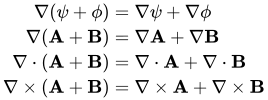
一次微分恒等式 スカラー場 、 およびベクトル場 、については 、次の微分恒等式が成り立ちます。
ψ
{\displaystyle \psi }
ϕ
{\displaystyle \phi }
A
{\displaystyle \mathbf {A} }
B
{\displaystyle \mathbf {B} }
分配法則
∇
(
ψ
+
ϕ
)
=
∇
ψ
+
∇
ϕ
∇
(
A
+
B
)
=
∇
A
+
∇
B
∇
⋅
(
A
+
B
)
=
∇
⋅
A
+
∇
⋅
B
∇
×
(
A
+
B
)
=
∇
×
A
+
∇
×
B
{\displaystyle {\begin{aligned}\nabla (\psi +\phi )&=\nabla \psi +\nabla \phi \\\nabla (\mathbf {A} +\mathbf {B} )&=\nabla \mathbf {A} +\nabla \mathbf {B} \\\nabla \cdot (\mathbf {A} +\mathbf {B} )&=\nabla \cdot \mathbf {A} +\nabla \cdot \mathbf {B} \\\nabla \times (\mathbf {A} +\mathbf {B} )&=\nabla \times \mathbf {A} +\nabla \times \mathbf {B} \end{aligned}}}
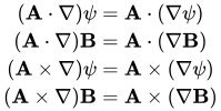
第一微分結合法則
(
A
⋅
∇
)
ψ
=
A
⋅
(
∇
ψ
)
(
A
⋅
∇
)
B
=
A
⋅
(
∇
B
)
(
A
×
∇
)
ψ
=
A
×
(
∇
ψ
)
(
A
×
∇
)
B
=
A
×
(
∇
B
)
{\displaystyle {\begin{aligned}(\mathbf {A} \cdot \nabla )\psi &=\mathbf {A} \cdot (\nabla \psi )\\(\mathbf {A} \cdot \nabla )\mathbf {B} &=\mathbf {A} \cdot (\nabla \mathbf {B} )\\(\mathbf {A} \times \nabla )\psi &=\mathbf {A} \times (\nabla \psi )\\(\mathbf {A} \times \nabla )\mathbf {B} &=\mathbf {A} \times (\nabla \mathbf {B} )\end{aligned}}}
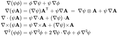
スカラーによる乗算の積の規則 一変数 微積分における 積分則 の一般化は次のようになります 。
∇
(
ψ
ϕ
)
=
ϕ
∇
ψ
+
ψ
∇
ϕ
∇
(
ψ
A
)
=
(
∇
ψ
)
A
T
+
ψ
∇
A
=
∇
ψ
⊗
A
+
ψ
∇
A
∇
⋅
(
ψ
A
)
=
ψ
∇
⋅
A
+
(
∇
ψ
)
⋅
A
∇
×
(
ψ
A
)
=
ψ
∇
×
A
+
(
∇
ψ
)
×
A
∇
2
(
ψ
ϕ
)
=
ψ
∇
2
ϕ
+
2
∇
ψ
⋅
∇
ϕ
+
ϕ
∇
2
ψ
{\displaystyle {\begin{aligned}\nabla (\psi \phi )&=\phi \,\nabla \psi +\psi \,\nabla \phi \\\nabla (\psi \mathbf {A} )&=(\nabla \psi )\mathbf {A} ^{\textsf {T}}+\psi \nabla \mathbf {A} \ =\ \nabla \psi \otimes \mathbf {A} +\psi \,\nabla \mathbf {A} \\\nabla \cdot (\psi \mathbf {A} )&=\psi \,\nabla {\cdot }\mathbf {A} +(\nabla \psi )\,{\cdot }\mathbf {A} \\\nabla {\times }(\psi \mathbf {A} )&=\psi \,\nabla {\times }\mathbf {A} +(\nabla \psi ){\times }\mathbf {A} \\\nabla ^{2}(\psi \phi )&=\psi \,\nabla ^{2\!}\phi +2\,\nabla \!\psi \cdot \!\nabla \phi +\phi \,\nabla ^{2\!}\psi \end{aligned}}}
スカラーによる除算の商規則
∇
(
ψ
ϕ
)
=
ϕ
∇
ψ
−
ψ
∇
ϕ
ϕ
2
∇
(
A
ϕ
)
=
ϕ
∇
A
−
∇
ϕ
⊗
A
ϕ
2
∇
⋅
(
A
ϕ
)
=
ϕ
∇
⋅
A
−
∇
ϕ
⋅
A
ϕ
2
∇
×
(
A
ϕ
)
=
ϕ
∇
×
A
−
∇
ϕ
×
A
ϕ
2
∇
2
(
ψ
ϕ
)
=
ϕ
∇
2
ψ
−
2
ϕ
∇
(
ψ
ϕ
)
⋅
∇
ϕ
−
ψ
∇
2
ϕ
ϕ
2
{\displaystyle {\begin{aligned}\nabla \left({\frac {\psi }{\phi }}\right)&={\frac {\phi \,\nabla \psi -\psi \,\nabla \phi }{\phi ^{2}}}\\[1em]\nabla \left({\frac {\mathbf {A} }{\phi }}\right)&={\frac {\phi \,\nabla \mathbf {A} -\nabla \phi \otimes \mathbf {A} }{\phi ^{2}}}\\[1em]\nabla \cdot \left({\frac {\mathbf {A} }{\phi }}\right)&={\frac {\phi \,\nabla {\cdot }\mathbf {A} -\nabla \!\phi \cdot \mathbf {A} }{\phi ^{2}}}\\[1em]\nabla \times \left({\frac {\mathbf {A} }{\phi }}\right)&={\frac {\phi \,\nabla {\times }\mathbf {A} -\nabla \!\phi \,{\times }\,\mathbf {A} }{\phi ^{2}}}\\[1em]\nabla ^{2}\left({\frac {\psi }{\phi }}\right)&={\frac {\phi \,\nabla ^{2\!}\psi -2\,\phi \,\nabla \!\left({\frac {\psi }{\phi }}\right)\cdot \!\nabla \phi -\psi \,\nabla ^{2\!}\phi }{\phi ^{2}}}\end{aligned}}}
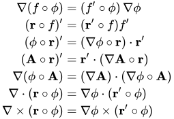
チェーンルール をスカラーからスカラーへの 1 変数関数、 パラメーター化された 曲線 、 ベクトルからスカラーへの関数、および ベクトル場と します。多変数 連鎖律 の特殊なケースとして次のものがあります。
f
(
x
)
{\displaystyle f(x)}
r
(
t
)
=
(
x
1
(
t
)
,
…
,
x
n
(
t
)
)
{\displaystyle \mathbf {r} (t)=(x_{1}(t),\ldots ,x_{n}(t))}
ϕ
:
R
n
→
R
{\displaystyle \phi \!:\mathbb {R} ^{n}\to \mathbb {R} }
A
:
R
n
→
R
n
{\displaystyle \mathbf {A} \!:\mathbb {R} ^{n}\to \mathbb {R} ^{n}}
∇
(
f
∘
ϕ
)
=
(
f
′
∘
ϕ
)
∇
ϕ
(
r
∘
f
)
′
=
(
r
′
∘
f
)
f
′
(
ϕ
∘
r
)
′
=
(
∇
ϕ
∘
r
)
⋅
r
′
(
A
∘
r
)
′
=
r
′
⋅
(
∇
A
∘
r
)
∇
(
ϕ
∘
A
)
=
(
∇
A
)
⋅
(
∇
ϕ
∘
A
)
∇
⋅
(
r
∘
ϕ
)
=
∇
ϕ
⋅
(
r
′
∘
ϕ
)
∇
×
(
r
∘
ϕ
)
=
∇
ϕ
×
(
r
′
∘
ϕ
)
{\displaystyle {\begin{aligned}\nabla (f\circ \phi )&=\left(f'\circ \phi \right)\nabla \phi \\(\mathbf {r} \circ f)'&=(\mathbf {r} '\circ f)f'\\(\phi \circ \mathbf {r} )'&=(\nabla \phi \circ \mathbf {r} )\cdot \mathbf {r} '\\(\mathbf {A} \circ \mathbf {r} )'&=\mathbf {r} '\cdot (\nabla \mathbf {A} \circ \mathbf {r} )\\\nabla (\phi \circ \mathbf {A} )&=(\nabla \mathbf {A} )\cdot (\nabla \phi \circ \mathbf {A} )\\\nabla \cdot (\mathbf {r} \circ \phi )&=\nabla \phi \cdot (\mathbf {r} '\circ \phi )\\\nabla \times (\mathbf {r} \circ \phi )&=\nabla \phi \times (\mathbf {r} '\circ \phi )\end{aligned}}}
ベクトル変換の場合、 次のようになります。
x
:
R
n
→
R
n
{\displaystyle \mathbf {x} \!:\mathbb {R} ^{n}\to \mathbb {R} ^{n}}
∇
⋅
(
A
∘
x
)
=
t
r
(
(
∇
x
)
⋅
(
∇
A
∘
x
)
)
{\displaystyle \nabla \cdot (\mathbf {A} \circ \mathbf {x} )=\mathrm {tr} \left((\nabla \mathbf {x} )\cdot (\nabla \mathbf {A} \circ \mathbf {x} )\right)}
ここでは、2 つの 2 次テンソルのドット積の
トレース を取得します。これは、それらの行列の積に対応します。
ドット積の規則
∇
(
A
⋅
B
)
=
(
A
⋅
∇
)
B
+
(
B
⋅
∇
)
A
+
A
×
(
∇
×
B
)
+
B
×
(
∇
×
A
)
=
A
⋅
J
B
+
B
⋅
J
A
=
(
∇
B
)
⋅
A
+
(
∇
A
)
⋅
B
{\displaystyle {\begin{aligned}\nabla (\mathbf {A} \cdot \mathbf {B} )&\ =\ (\mathbf {A} \cdot \nabla )\mathbf {B} \,+\,(\mathbf {B} \cdot \nabla )\mathbf {A} \,+\,\mathbf {A} {\times }(\nabla {\times }\mathbf {B} )\,+\,\mathbf {B} {\times }(\nabla {\times }\mathbf {A} )\\&\ =\ \mathbf {A} \cdot \mathbf {J} _{\mathbf {B} }+\mathbf {B} \cdot \mathbf {J} _{\mathbf {A} }\ =\ (\nabla \mathbf {B} )\cdot \mathbf {A} \,+\,(\nabla \mathbf {A} )\cdot \mathbf {B} \end{aligned}}}
ここで は ベクトル場 の ヤコビ行列 を表します 。
J
A
=
(
∇
A
)
T
=
(
∂
A
i
/
∂
x
j
)
i
j
{\displaystyle \mathbf {J} _{\mathbf {A} }=(\nabla \!\mathbf {A} )^{\textsf {T}}=(\partial A_{i}/\partial x_{j})_{ij}}
A
=
(
A
1
,
…
,
A
n
)
{\displaystyle \mathbf {A} =(A_{1},\ldots ,A_{n})}
あるいは、ファインマンの添え字表記法を使うと、
∇
(
A
⋅
B
)
=
∇
A
(
A
⋅
B
)
+
∇
B
(
A
⋅
B
)
.
{\displaystyle \nabla (\mathbf {A} \cdot \mathbf {B} )=\nabla _{\mathbf {A} }(\mathbf {A} \cdot \mathbf {B} )+\nabla _{\mathbf {B} }(\mathbf {A} \cdot \mathbf {B} )\ .}
こちらのノートを参照。 [4]
特別な場合として、 A = B の とき、
1
2
∇
(
A
⋅
A
)
=
A
⋅
J
A
=
(
∇
A
)
⋅
A
=
(
A
⋅
∇
)
A
+
A
×
(
∇
×
A
)
=
A
∇
A
.
{\displaystyle {\tfrac {1}{2}}\nabla \left(\mathbf {A} \cdot \mathbf {A} \right)\ =\ \mathbf {A} \cdot \mathbf {J} _{\mathbf {A} }\ =\ (\nabla \mathbf {A} )\cdot \mathbf {A} \ =\ (\mathbf {A} {\cdot }\nabla )\mathbf {A} \,+\,\mathbf {A} {\times }(\nabla {\times }\mathbf {A} )\ =\ A\nabla A.}
ドット積 公式の リーマン多様体 への一般化は 、ベクトル場を微分してベクトル値 1 形式を与える リーマン接続 の定義特性です 。
外積のルール
∇
(
A
×
B
)
=
(
∇
A
)
×
B
−
(
∇
B
)
×
A
∇
⋅
(
A
×
B
)
=
(
∇
×
A
)
⋅
B
−
A
⋅
(
∇
×
B
)
∇
×
(
A
×
B
)
=
A
(
∇
⋅
B
)
−
B
(
∇
⋅
A
)
+
(
B
⋅
∇
)
A
−
(
A
⋅
∇
)
B
=
A
(
∇
⋅
B
)
+
(
B
⋅
∇
)
A
−
(
B
(
∇
⋅
A
)
+
(
A
⋅
∇
)
B
)
=
∇
⋅
(
B
A
T
)
−
∇
⋅
(
A
B
T
)
=
∇
⋅
(
B
A
T
−
A
B
T
)
A
×
(
∇
×
B
)
=
∇
B
(
A
⋅
B
)
−
(
A
⋅
∇
)
B
=
A
⋅
J
B
−
(
A
⋅
∇
)
B
=
(
∇
B
)
⋅
A
−
A
⋅
(
∇
B
)
=
A
⋅
(
J
B
−
J
B
T
)
(
A
×
∇
)
×
B
=
(
∇
B
)
⋅
A
−
A
(
∇
⋅
B
)
=
A
×
(
∇
×
B
)
+
(
A
⋅
∇
)
B
−
A
(
∇
⋅
B
)
(
A
×
∇
)
⋅
B
=
A
⋅
(
∇
×
B
)
{\displaystyle {\begin{aligned}\nabla (\mathbf {A} \times \mathbf {B} )&\ =\ (\nabla \mathbf {A} )\times \mathbf {B} \,-\,(\nabla \mathbf {B} )\times \mathbf {A} \\[5pt]\nabla \cdot (\mathbf {A} \times \mathbf {B} )&\ =\ (\nabla {\times }\mathbf {A} )\cdot \mathbf {B} \,-\,\mathbf {A} \cdot (\nabla {\times }\mathbf {B} )\\[5pt]\nabla \times (\mathbf {A} \times \mathbf {B} )&\ =\ \mathbf {A} (\nabla {\cdot }\mathbf {B} )\,-\,\mathbf {B} (\nabla {\cdot }\mathbf {A} )\,+\,(\mathbf {B} {\cdot }\nabla )\mathbf {A} \,-\,(\mathbf {A} {\cdot }\nabla )\mathbf {B} \\[2pt]&\ =\ \mathbf {A} (\nabla {\cdot }\mathbf {B} )\,+\,(\mathbf {B} {\cdot }\nabla )\mathbf {A} \,-\,(\mathbf {B} (\nabla {\cdot }\mathbf {A} )\,+\,(\mathbf {A} {\cdot }\nabla )\mathbf {B} )\\[2pt]&\ =\ \nabla {\cdot }\left(\mathbf {B} \mathbf {A} ^{\textsf {T}}\right)\,-\,\nabla {\cdot }\left(\mathbf {A} \mathbf {B} ^{\textsf {T}}\right)\\[2pt]&\ =\ \nabla {\cdot }\left(\mathbf {B} \mathbf {A} ^{\textsf {T}}\,-\,\mathbf {A} \mathbf {B} ^{\textsf {T}}\right)\\[5pt]\mathbf {A} \times (\nabla \times \mathbf {B} )&\ =\ \nabla _{\mathbf {B} }(\mathbf {A} {\cdot }\mathbf {B} )\,-\,(\mathbf {A} {\cdot }\nabla )\mathbf {B} \\[2pt]&\ =\ \mathbf {A} \cdot \mathbf {J} _{\mathbf {B} }\,-\,(\mathbf {A} {\cdot }\nabla )\mathbf {B} \\[2pt]&\ =\ (\nabla \mathbf {B} )\cdot \mathbf {A} \,-\,\mathbf {A} \cdot (\nabla \mathbf {B} )\\[2pt]&\ =\ \mathbf {A} \cdot (\mathbf {J} _{\mathbf {B} }\,-\,\mathbf {J} _{\mathbf {B} }^{\textsf {T}})\\[5pt](\mathbf {A} \times \nabla )\times \mathbf {B} &\ =\ (\nabla \mathbf {B} )\cdot \mathbf {A} \,-\,\mathbf {A} (\nabla {\cdot }\mathbf {B} )\\[2pt]&\ =\ \mathbf {A} \times (\nabla \times \mathbf {B} )\,+\,(\mathbf {A} {\cdot }\nabla )\mathbf {B} \,-\,\mathbf {A} (\nabla {\cdot }\mathbf {B} )\\[5pt](\mathbf {A} \times \nabla )\cdot \mathbf {B} &\ =\ \mathbf {A} \cdot (\nabla {\times }\mathbf {B} )\end{aligned}}}
行列は 反対称であることに注意してください。
J
B
−
J
B
T
{\displaystyle \mathbf {J} _{\mathbf {B} }\,-\,\mathbf {J} _{\mathbf {B} }^{\textsf {T}}}
2次導関数の同一性
回転の発散はゼロ 任意 の連続2回微分可能な ベクトル場 A の回転の 発散 は 常にゼロです。
∇
⋅
(
∇
×
A
)
=
0
{\displaystyle \nabla \cdot (\nabla \times \mathbf {A} )=0}
これは、 De Rham 連鎖複体 における 外微分 の二乗が消失する特殊なケースです 。
勾配の発散はラプラシアンである スカラー場のラプラシアン は その勾配の発散です。
結果はスカラー量です。
Δ
ψ
=
∇
2
ψ
=
∇
⋅
(
∇
ψ
)
{\displaystyle \Delta \psi =\nabla ^{2}\psi =\nabla \cdot (\nabla \psi )}
発散の発散は定義されていない ベクトル場A の発散は スカラーであり、スカラー量の発散は定義されていない。したがって、
∇
⋅
(
∇
⋅
A
)
is undefined.
{\displaystyle \nabla \cdot (\nabla \cdot \mathbf {A} ){\text{ is undefined.}}}
勾配のカールはゼロです 任意の連続的 に2回微分可能な スカラー場 (すなわち、 微分可能クラス )の 勾配 の 回転 は 常に ゼロベクトル です。
φ
{\displaystyle \varphi }
C
2
{\displaystyle C^{2}}
∇
×
(
∇
φ
)
=
0
.
{\displaystyle \nabla \times (\nabla \varphi )=\mathbf {0} .}
これは、シュワルツの定理 (混合偏微分の等式に関するクレローの定理とも呼ばれる)を使用して 直交座標系 で 表現することで簡単に証明できます。この結果は、 ド・ラーム 鎖複体 における 外微分 の2乗が消失する特殊なケースです 。
∇
×
(
∇
φ
)
{\displaystyle \nabla \times (\nabla \varphi )}
カールのカール
∇
×
(
∇
×
A
)
=
∇
(
∇
⋅
A
)
−
∇
2
A
{\displaystyle \nabla \times \left(\nabla \times \mathbf {A} \right)\ =\ \nabla (\nabla {\cdot }\mathbf {A} )\,-\,\nabla ^{2\!}\mathbf {A} }
ここで∇2 は ベクトル場 A上で作用する ベクトルラプラシアン です 。
発散曲線は定義されていない ベクトル場 A の発散 は スカラーであり、スカラー量の回転は定義されていない。したがって、
∇
×
(
∇
⋅
A
)
is undefined.
{\displaystyle \nabla \times (\nabla \cdot \mathbf {A} ){\text{ is undefined.}}}
2次微分結合特性
(
∇
⋅
∇
)
ψ
=
∇
⋅
(
∇
ψ
)
=
∇
2
ψ
(
∇
⋅
∇
)
A
=
∇
⋅
(
∇
A
)
=
∇
2
A
(
∇
×
∇
)
ψ
=
∇
×
(
∇
ψ
)
=
0
(
∇
×
∇
)
A
=
∇
×
(
∇
A
)
=
0
{\displaystyle {\begin{aligned}(\nabla \cdot \nabla )\psi &=\nabla \cdot (\nabla \psi )=\nabla ^{2}\psi \\(\nabla \cdot \nabla )\mathbf {A} &=\nabla \cdot (\nabla \mathbf {A} )=\nabla ^{2}\mathbf {A} \\(\nabla \times \nabla )\psi &=\nabla \times (\nabla \psi )=\mathbf {0} \\(\nabla \times \nabla )\mathbf {A} &=\nabla \times (\nabla \mathbf {A} )=\mathbf {0} \end{aligned}}}
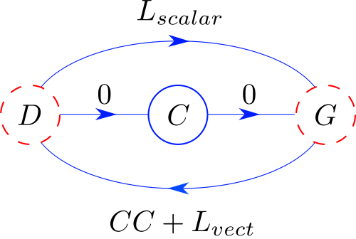
DCG チャート: 2 次導関数のいくつかのルール。
記憶術 右の図は、これらのアイデンティティの一部を記憶するためのものです。使用される略語は次のとおりです。
D: 発散、 C: カール、 G: グラデーション、 L: ラプラシアン、 CC: カールのカール。 各矢印には、恒等式の結果、具体的には矢印の末尾の演算子を矢印の先頭の演算子に適用した結果がラベル付けされています。中央の青い円は回転が存在することを意味し、他の 2 つの赤い円 (破線) は DD と GG が存在しないことを意味します。
重要なアイデンティティの概要
差別化
勾配
∇
(
ψ
+
ϕ
)
=
∇
ψ
+
∇
ϕ
{\displaystyle \nabla (\psi +\phi )=\nabla \psi +\nabla \phi }
∇
(
ψ
ϕ
)
=
ϕ
∇
ψ
+
ψ
∇
ϕ
{\displaystyle \nabla (\psi \phi )=\phi \nabla \psi +\psi \nabla \phi }
∇
(
ψ
A
)
=
∇
ψ
⊗
A
+
ψ
∇
A
{\displaystyle \nabla (\psi \mathbf {A} )=\nabla \psi \otimes \mathbf {A} +\psi \nabla \mathbf {A} }
∇
(
A
⋅
B
)
=
(
A
⋅
∇
)
B
+
(
B
⋅
∇
)
A
+
A
×
(
∇
×
B
)
+
B
×
(
∇
×
A
)
{\displaystyle \nabla (\mathbf {A} \cdot \mathbf {B} )=(\mathbf {A} \cdot \nabla )\mathbf {B} +(\mathbf {B} \cdot \nabla )\mathbf {A} +\mathbf {A} \times (\nabla \times \mathbf {B} )+\mathbf {B} \times (\nabla \times \mathbf {A} )}
発散
∇
⋅
(
A
+
B
)
=
∇
⋅
A
+
∇
⋅
B
{\displaystyle \nabla \cdot (\mathbf {A} +\mathbf {B} )=\nabla \cdot \mathbf {A} +\nabla \cdot \mathbf {B} }
∇
⋅
(
ψ
A
)
=
ψ
∇
⋅
A
+
A
⋅
∇
ψ
{\displaystyle \nabla \cdot \left(\psi \mathbf {A} \right)=\psi \nabla \cdot \mathbf {A} +\mathbf {A} \cdot \nabla \psi }
∇
⋅
(
A
×
B
)
=
(
∇
×
A
)
⋅
B
−
(
∇
×
B
)
⋅
A
{\displaystyle \nabla \cdot \left(\mathbf {A} \times \mathbf {B} \right)=(\nabla \times \mathbf {A} )\cdot \mathbf {B} -(\nabla \times \mathbf {B} )\cdot \mathbf {A} }
カール
∇
×
(
A
+
B
)
=
∇
×
A
+
∇
×
B
{\displaystyle \nabla \times (\mathbf {A} +\mathbf {B} )=\nabla \times \mathbf {A} +\nabla \times \mathbf {B} }
∇
×
(
ψ
A
)
=
ψ
(
∇
×
A
)
−
(
A
×
∇
)
ψ
=
ψ
(
∇
×
A
)
+
(
∇
ψ
)
×
A
{\displaystyle \nabla \times \left(\psi \mathbf {A} \right)=\psi \,(\nabla \times \mathbf {A} )-(\mathbf {A} \times \nabla )\psi =\psi \,(\nabla \times \mathbf {A} )+(\nabla \psi )\times \mathbf {A} }
∇
×
(
ψ
∇
ϕ
)
=
∇
ψ
×
∇
ϕ
{\displaystyle \nabla \times \left(\psi \nabla \phi \right)=\nabla \psi \times \nabla \phi }
∇
×
(
A
×
B
)
=
A
(
∇
⋅
B
)
−
B
(
∇
⋅
A
)
+
(
B
⋅
∇
)
A
−
(
A
⋅
∇
)
B
{\displaystyle \nabla \times \left(\mathbf {A} \times \mathbf {B} \right)=\mathbf {A} \left(\nabla \cdot \mathbf {B} \right)-\mathbf {B} \left(\nabla \cdot \mathbf {A} \right)+\left(\mathbf {B} \cdot \nabla \right)\mathbf {A} -\left(\mathbf {A} \cdot \nabla \right)\mathbf {B} }
[5]
ベクトルドットデル演算子
(
A
⋅
∇
)
B
=
1
2
[
∇
(
A
⋅
B
)
−
∇
×
(
A
×
B
)
−
B
×
(
∇
×
A
)
−
A
×
(
∇
×
B
)
−
B
(
∇
⋅
A
)
+
A
(
∇
⋅
B
)
]
{\displaystyle (\mathbf {A} \cdot \nabla )\mathbf {B} ={\frac {1}{2}}{\bigg [}\nabla (\mathbf {A} \cdot \mathbf {B} )-\nabla \times (\mathbf {A} \times \mathbf {B} )-\mathbf {B} \times (\nabla \times \mathbf {A} )-\mathbf {A} \times (\nabla \times \mathbf {B} )-\mathbf {B} (\nabla \cdot \mathbf {A} )+\mathbf {A} (\nabla \cdot \mathbf {B} ){\bigg ]}}
[6]
(
A
⋅
∇
)
A
=
1
2
∇
|
A
|
2
−
A
×
(
∇
×
A
)
=
1
2
∇
|
A
|
2
+
(
∇
×
A
)
×
A
{\displaystyle (\mathbf {A} \cdot \nabla )\mathbf {A} ={\frac {1}{2}}\nabla |\mathbf {A} |^{2}-\mathbf {A} \times (\nabla \times \mathbf {A} )={\frac {1}{2}}\nabla |\mathbf {A} |^{2}+(\nabla \times \mathbf {A} )\times \mathbf {A} }
A
⋅
∇
(
B
⋅
B
)
=
2
B
⋅
(
A
⋅
∇
)
B
{\displaystyle \mathbf {A} \cdot \nabla (\mathbf {B} \cdot \mathbf {B} )=2\mathbf {B} \cdot (\mathbf {A} \cdot \nabla )\mathbf {B} }
2次導関数
∇
⋅
(
∇
×
A
)
=
0
{\displaystyle \nabla \cdot (\nabla \times \mathbf {A} )=0}
∇
×
(
∇
ψ
)
=
0
{\displaystyle \nabla \times (\nabla \psi )=\mathbf {0} }
∇
⋅
(
∇
ψ
)
=
∇
2
ψ
{\displaystyle \nabla \cdot (\nabla \psi )=\nabla ^{2}\psi }
( スカラーラプラシアン )
∇
(
∇
⋅
A
)
−
∇
×
(
∇
×
A
)
=
∇
2
A
{\displaystyle \nabla \left(\nabla \cdot \mathbf {A} \right)-\nabla \times \left(\nabla \times \mathbf {A} \right)=\nabla ^{2}\mathbf {A} }
( ベクトルラプラシアン )
∇
⋅
(
ϕ
∇
ψ
)
=
ϕ
∇
2
ψ
+
∇
ϕ
⋅
∇
ψ
{\displaystyle \nabla \cdot (\phi \nabla \psi )=\phi \nabla ^{2}\psi +\nabla \phi \cdot \nabla \psi }
ψ
∇
2
ϕ
−
ϕ
∇
2
ψ
=
∇
⋅
(
ψ
∇
ϕ
−
ϕ
∇
ψ
)
{\displaystyle \psi \nabla ^{2}\phi -\phi \nabla ^{2}\psi =\nabla \cdot \left(\psi \nabla \phi -\phi \nabla \psi \right)}
∇
2
(
ϕ
ψ
)
=
ϕ
∇
2
ψ
+
2
(
∇
ϕ
)
⋅
(
∇
ψ
)
+
(
∇
2
ϕ
)
ψ
{\displaystyle \nabla ^{2}(\phi \psi )=\phi \nabla ^{2}\psi +2(\nabla \phi )\cdot (\nabla \psi )+\left(\nabla ^{2}\phi \right)\psi }
∇
2
(
ψ
A
)
=
A
∇
2
ψ
+
2
(
∇
ψ
⋅
∇
)
A
+
ψ
∇
2
A
{\displaystyle \nabla ^{2}(\psi \mathbf {A} )=\mathbf {A} \nabla ^{2}\psi +2(\nabla \psi \cdot \nabla )\mathbf {A} +\psi \nabla ^{2}\mathbf {A} }
∇
2
(
A
⋅
B
)
=
A
⋅
∇
2
B
−
B
⋅
∇
2
A
+
2
∇
⋅
(
(
B
⋅
∇
)
A
+
B
×
(
∇
×
A
)
)
{\displaystyle \nabla ^{2}(\mathbf {A} \cdot \mathbf {B} )=\mathbf {A} \cdot \nabla ^{2}\mathbf {B} -\mathbf {B} \cdot \nabla ^{2}\!\mathbf {A} +2\nabla \cdot ((\mathbf {B} \cdot \nabla )\mathbf {A} +\mathbf {B} \times (\nabla \times \mathbf {A} ))}
( グリーンのベクトル恒等式 )
3次導関数
∇
2
(
∇
ψ
)
=
∇
(
∇
⋅
(
∇
ψ
)
)
=
∇
(
∇
2
ψ
)
{\displaystyle \nabla ^{2}(\nabla \psi )=\nabla (\nabla \cdot (\nabla \psi ))=\nabla \left(\nabla ^{2}\psi \right)}
∇
2
(
∇
⋅
A
)
=
∇
⋅
(
∇
(
∇
⋅
A
)
)
=
∇
⋅
(
∇
2
A
)
{\displaystyle \nabla ^{2}(\nabla \cdot \mathbf {A} )=\nabla \cdot (\nabla (\nabla \cdot \mathbf {A} ))=\nabla \cdot \left(\nabla ^{2}\mathbf {A} \right)}
∇
2
(
∇
×
A
)
=
−
∇
×
(
∇
×
(
∇
×
A
)
)
=
∇
×
(
∇
2
A
)
{\displaystyle \nabla ^{2}(\nabla \times \mathbf {A} )=-\nabla \times (\nabla \times (\nabla \times \mathbf {A} ))=\nabla \times \left(\nabla ^{2}\mathbf {A} \right)}
統合 以下では、 波記号 ∂ は 表面または立体
の 「 境界」を意味します。
表面積積分 以下の表面積積分定理において、 V は対応する2次元 境界 S = ∂ V ( 閉じた面 )を持つ3次元体積を表します 。
∂
V
{\displaystyle \scriptstyle \partial V}
ψ
d
S
=
∭
V
∇
ψ
d
V
{\displaystyle \psi \,d\mathbf {S} \ =\ \iiint _{V}\nabla \psi \,dV}
∂
V
{\displaystyle \scriptstyle \partial V}
A
⋅
d
S
=
∭
V
∇
⋅
A
d
V
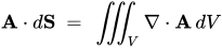
{\displaystyle \mathbf {A} \cdot d\mathbf {S} \ =\ \iiint _{V}\nabla \cdot \mathbf {A} \,dV}
( 発散定理 )
∂
V
{\displaystyle \scriptstyle \partial V}
A
×
d
S
=
−
∭
V
∇
×
A
d
V
{\displaystyle \mathbf {A} \times d\mathbf {S} \ =\ -\iiint _{V}\nabla \times \mathbf {A} \,dV}
∂
V
{\displaystyle \scriptstyle \partial V}
ψ
∇
φ
⋅
d
S
=
∭
V
(
ψ
∇
2
φ
+
∇
φ
⋅
∇
ψ
)
d
V
{\displaystyle \psi \nabla \!\varphi \cdot d\mathbf {S} \ =\ \iiint _{V}\left(\psi \nabla ^{2}\!\varphi +\nabla \!\varphi \cdot \nabla \!\psi \right)\,dV}
( グリーンの最初のアイデンティティ )
∂
V
{\displaystyle \scriptstyle \partial V}
(
ψ
∇
φ
−
φ
∇
ψ
)
⋅
d
S
=
{\displaystyle \left(\psi \nabla \!\varphi -\varphi \nabla \!\psi \right)\cdot d\mathbf {S} \ =\ }
∂
V
{\displaystyle \scriptstyle \partial V}
(
ψ
∂
φ
∂
n
−
φ
∂
ψ
∂
n
)
d
S
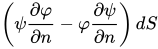
{\displaystyle \left(\psi {\frac {\partial \varphi }{\partial n}}-\varphi {\frac {\partial \psi }{\partial n}}\right)dS}
=
∭
V
(
ψ
∇
2
φ
−
φ
∇
2
ψ
)
d
V
{\displaystyle \displaystyle \ =\ \iiint _{V}\left(\psi \nabla ^{2}\!\varphi -\varphi \nabla ^{2}\!\psi \right)\,dV}
( グリーンの第二のアイデンティティ )
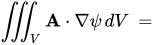
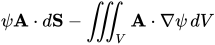
∭
V
A
⋅
∇
ψ
d
V
=
{\displaystyle \iiint _{V}\mathbf {A} \cdot \nabla \psi \,dV\ =\ }
∂
V
{\displaystyle \scriptstyle \partial V}
ψ
A
⋅
d
S
−
∭
V
ψ
∇
⋅
A
d
V
{\displaystyle \psi \mathbf {A} \cdot d\mathbf {S} -\iiint _{V}\psi \nabla \cdot \mathbf {A} \,dV}
( 部分積分 )
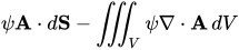
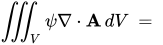
∭
V
ψ
∇
⋅
A
d
V
=
{\displaystyle \iiint _{V}\psi \nabla \cdot \mathbf {A} \,dV\ =\ }
∂
V
{\displaystyle \scriptstyle \partial V}
ψ
A
⋅
d
S
−
∭
V
A
⋅
∇
ψ
d
V
{\displaystyle \psi \mathbf {A} \cdot d\mathbf {S} -\iiint _{V}\mathbf {A} \cdot \nabla \psi \,dV}
( 部分積分 )
∭
V
A
⋅
(
∇
×
B
)
d
V
=
−
{\displaystyle \iiint _{V}\mathbf {A} \cdot \left(\nabla \times \mathbf {B} \right)\,dV\ =\ -}
∂
V
{\displaystyle \scriptstyle \partial V}
(
A
×
B
)
⋅
d
S
+
∭
V
(
∇
×
A
)
⋅
B
d
V
{\displaystyle \left(\mathbf {A} \times \mathbf {B} \right)\cdot d\mathbf {S} +\iiint _{V}\left(\nabla \times \mathbf {A} \right)\cdot \mathbf {B} \,dV}
( 部分積分 )
∂
V
{\displaystyle \scriptstyle \partial V}
A
×
(
d
S
⋅
(
B
C
T
)
)
=
∭
V
A
×
(
∇
⋅
(
B
C
T
)
)
d
V
+
∭
V
B
⋅
(
∇
A
)
×
C
d
V
{\displaystyle \mathbf {A} \times \left(d\mathbf {S} \cdot \left(\mathbf {B} \mathbf {C} ^{\textsf {T}}\right)\right)\ =\ \iiint _{V}\mathbf {A} \times \left(\nabla \cdot \left(\mathbf {B} \mathbf {C} ^{\textsf {T}}\right)\right)\,dV+\iiint _{V}\mathbf {B} \cdot (\nabla \mathbf {A} )\times \mathbf {C} \,dV}
[7]
∭
V
(
∇
⋅
B
+
B
⋅
∇
)
A
d
V
=
{\displaystyle \iiint _{V}\left(\nabla \cdot \mathbf {B} +\mathbf {B} \cdot \nabla \right)\mathbf {A} \,dV\ =\ }
∂
V
{\displaystyle \scriptstyle \partial V}
(
B
⋅
d
S
)
A
{\displaystyle \left(\mathbf {B} \cdot d\mathbf {S} \right)\mathbf {A} }
[8]
曲線面積分 以下の曲線-面積分定理において、 S は対応する 1d 境界 C = ∂ S ( 閉曲線 )を持つ 2d 開面を表します 。
∮
∂
S
A
⋅
d
ℓ
=
∬
S
(
∇
×
A
)
⋅
d
S
{\displaystyle \oint _{\partial S}\mathbf {A} \cdot d{\boldsymbol {\ell }}\ =\ \iint _{S}\left(\nabla \times \mathbf {A} \right)\cdot d\mathbf {S} }
( ストークスの定理 )
∮
∂
S
ψ
d
ℓ
=
−
∬
S
∇
ψ
×
d
S
{\displaystyle \oint _{\partial S}\psi \,d{\boldsymbol {\ell }}\ =\ -\iint _{S}\nabla \psi \times d\mathbf {S} }
∮
∂
S
A
×
d
ℓ
=
−
∬
S
(
∇
A
−
(
∇
⋅
A
)
1
)
⋅
d
S
=
−
∬
S
(
d
S
×
∇
)
×
A
{\displaystyle \oint _{\partial S}\mathbf {A} \times d{\boldsymbol {\ell }}\ =\ -\iint _{S}\left(\nabla \mathbf {A} -(\nabla \cdot \mathbf {A} )\mathbf {1} \right)\cdot d\mathbf {S} \ =\ -\iint _{S}\left(d\mathbf {S} \times \nabla \right)\times \mathbf {A} }
∮
∂
S
A
×
(
B
×
d
ℓ
)
=
∬
S
(
∇
×
(
A
B
T
)
)
⋅
d
S
+
∬
S
(
∇
⋅
(
B
A
T
)
)
×
d
S
{\displaystyle \oint _{\partial S}\mathbf {A} \times (\mathbf {B} \times d{\boldsymbol {\ell }})\ =\ \iint _{S}\left(\nabla \times \left(\mathbf {A} \mathbf {B} ^{\textsf {T}}\right)\right)\cdot d\mathbf {S} +\iint _{S}\left(\nabla \cdot \left(\mathbf {B} \mathbf {A} ^{\textsf {T}}\right)\right)\times d\mathbf {S} }
[9]
∮
∂
S
(
B
⋅
d
ℓ
)
A
=
∬
S
(
d
S
⋅
[
∇
×
B
−
B
×
∇
]
)
A
{\displaystyle \oint _{\partial S}(\mathbf {B} \cdot d{\boldsymbol {\ell }})\mathbf {A} =\iint _{S}(d\mathbf {S} \cdot \left[\nabla \times \mathbf {B} -\mathbf {B} \times \nabla \right])\mathbf {A} }
[10] 閉曲線の周りの 時計回りの積分は、同じ線積分の反時計回りの負の値です( 定積分 における極限の交換に似ています )。
∂
S
{\displaystyle {\scriptstyle \partial S}}
A
⋅
d
ℓ
=
−
{\displaystyle \mathbf {A} \cdot d{\boldsymbol {\ell }}=-}
∂
S
{\displaystyle {\scriptstyle \partial S}}
A
⋅
d
ℓ
.
{\displaystyle \mathbf {A} \cdot d{\boldsymbol {\ell }}.}
端点曲線積分 次の端点曲線積分定理において、 P は 符号付き 0d 境界点を持つ 1d 開路を表し 、 P に沿った積分は からまで です 。
q
−
p
=
∂
P
{\displaystyle \mathbf {q} -\mathbf {p} =\partial P}
p
{\displaystyle \mathbf {p} }
q
{\displaystyle \mathbf {q} }
ψ
|
∂
P
=
ψ
(
q
)
−
ψ
(
p
)
=
∫
P
∇
ψ
⋅
d
ℓ
{\displaystyle \psi |_{\partial P}=\psi (\mathbf {q} )-\psi (\mathbf {p} )=\int _{P}\nabla \psi \cdot d{\boldsymbol {\ell }}}
( 勾配定理 )
A
|
∂
P
=
A
(
q
)
−
A
(
p
)
=
∫
P
(
d
ℓ
⋅
∇
)
A
{\displaystyle \mathbf {A} |_{\partial P}=\mathbf {A} (\mathbf {q} )-\mathbf {A} (\mathbf {p} )=\int _{P}\left(d{\boldsymbol {\ell }}\cdot \nabla \right)\mathbf {A} }
A
|
∂
P
=
A
(
q
)
−
A
(
p
)
=
∫
P
(
∇
A
)
⋅
d
ℓ
+
∫
P
(
∇
×
A
)
×
d
ℓ
{\displaystyle \mathbf {A} |_{\partial P}=\mathbf {A} (\mathbf {q} )-\mathbf {A} (\mathbf {p} )=\int _{P}\left(\nabla \mathbf {A} \right)\cdot d{\boldsymbol {\ell }}+\int _{P}\left(\nabla \times \mathbf {A} \right)\times d{\boldsymbol {\ell }}}
テンソル積分 ベクトル積分定理のテンソル形式は、ベクトル(またはベクトルの1つ)をテンソルに置き換えることによって得られます。ただし、そのベクトルは、まず各積分関数の最も右側のベクトルとしてのみ現れるようにする必要があります。たとえば、ストークスの定理は次のようになります。
∮
∂
S
d
ℓ
⋅
T
=
∬
S
d
S
⋅
(
∇
×
T
)
{\displaystyle \oint _{\partial S}d{\boldsymbol {\ell }}\cdot \mathbf {T} \ =\ \iint _{S}d\mathbf {S} \cdot \left(\nabla \times \mathbf {T} \right)}
。 スカラー場はベクトルとして扱われ、ベクトルまたはテンソルに置き換えられることもある。例えば、グリーンの最初の恒等式は次のようになる。
∂
V
{\displaystyle \scriptstyle \partial V}
ψ
d
S
⋅
∇
A
=
∭
V
(
ψ
∇
2
A
+
∇
ψ
⋅
∇
A
)
d
V
{\displaystyle \psi \,d\mathbf {S} \cdot \nabla \!\mathbf {A} \ =\ \iiint _{V}\left(\psi \nabla ^{2}\!\mathbf {A} +\nabla \!\psi \cdot \nabla \!\mathbf {A} \right)\,dV}
。 代数式や微分式にも同様の規則が適用されます。代数式の場合は、代わりに最も左のベクトルの位置を使用することもできます。
参照
参考文献
^ ファインマン、RP; レイトン、RB; サンズ、M. (1964). ファインマン物理学講義 . アディソン・ウェスレー. 第2巻、p. 27–4. ISBN 0-8053-9049-9 。 ^ Kholmetskii, AL; Missevitch, OV (2005). 「相対性理論におけるファラデー誘導法則」p. 4. arXiv : physics/0504223 . ^ Doran, C. ; Lasenby, A. (2003). 物理学者のための幾何代数 . ケンブリッジ大学出版局. p. 169. ISBN 978-0-521-71595-9 。 ^ Kelly, P. (2013). 「第1.14章 テンソル計算1: テンソル場」 (PDF) 。力学講義ノート第3部: 連続体力学の基礎。オークランド大学。 2017年 12月7日 閲覧 。 ^ "lecture15.pdf" (PDF) . ^ クオ、ケネス K.; アチャリヤ、ラギニ (2012)。乱流および多相燃焼の応用。ホーボーケン、ニュージャージー州: ワイリー。p. 520。doi : 10.1002 / 9781118127575.app1。ISBN 9781118127575 . 2021年4月19日時点のオリジナルよりアーカイブ 。 2020年 4月19日 閲覧。 ^ PageとAdams、65~66ページ。 ^ ワングスネス、ロアルド・K.; クラウド、マイケル・J. (1986). 電磁場 (第2版)。ワイリー 。ISBN 978-0-471-81186-2 。 ^ Page, Leigh; Adams, Norman Ilsley, Jr. (1940). 電気力学. ニューヨーク: D. Van Nostrand Company, Inc. pp. 44–45, 式 (18-3). {{cite book}}: CS1 maint: multiple names: authors list (link)^ Pérez-Garrido, Antonio (2024). 「ベクトル計算のあまり使われない定理の復元と電磁気学の問題への応用」. American Journal of Physics . 92 (5): 354–359. arXiv : 2312.17268 . doi :10.1119/5.0182191.
さらに読む
バラニス、コンスタンティン A. (1989 年 5 月 23 日) 。Advanced Engineering Electromagnetics。ISBN 0-471-62194-3 。 Schey, HM (1997)。Div Grad Curl and all that: ベクトル計算に関する非公式テキスト 。WW Norton & Company。ISBN 0-393-96997-5 。 グリフィス、デイビッド・J. (1999)。 『電気力学入門 』、プレンティス・ホール、 ISBN 0-13-805326-X 。




















![{\displaystyle {\begin{aligned}\operatorname {curl} \mathbf {F} &=\nabla \times \mathbf {F} ={\begin{pmatrix}\displaystyle {\frac {\partial }{\partial x}},\ {\frac {\partial }{\partial y}},\ {\frac {\partial }{\partial z}}\end{pmatrix}}\times {\begin{pmatrix}F_{x},\ F_{y},\ F_{z}\end{pmatrix}}={\begin{vmatrix}\mathbf {i} &\mathbf {j} &\mathbf {k} \\{\frac {\partial }{\partial x}}&{\frac {\partial }{\partial y}}&{\frac {\partial }{\partial z}}\\F_{x}&F_{y}&F_{z}\end{vmatrix}}\\[1em]&=\left({\frac {\partial F_{z}}{\partial y}}-{\frac {\partial F_{y}}{\partial z}}\right)\mathbf {i} +\left({\frac {\partial F_{x}}{\partial z}}-{\frac {\partial F_{z}}{\partial x}}\right)\mathbf {j} +\left({\frac {\partial F_{y}}{\partial x}}-{\frac {\partial F_{x}}{\partial y}}\right)\mathbf {k} \end{aligned}}}](https://wikimedia.org/api/rest_v1/media/math/render/svg/8579a43f51c457ddcad8e559206bf6e1696b1419)













![{\displaystyle {\begin{aligned}\nabla \cdot (\mathbf {A} \times \mathbf {B} )&=\nabla _{\mathbf {A} }\cdot (\mathbf {A} \times \ mathbf {B} )+\nabla _{\mathbf {B} }\cdot (\mathbf {A} \times \mathbf {B} )\\[2pt]&=(\nabla _{\mathbf {A} }\times \mathbf {A} )\cdot \mathbf {B} +(\nabla _{\mathbf {B} }\倍 \mathbf {A} )\cdot \mathbf {B} \\[2pt]&=(\nabla _{\mathbf {A} }\times \mathbf {A} )\cdot \mathbf {B} -(\mathbf {A} \times \nabla _{\mathbf {B} })\cdot \mathbf {B} \\[2pt]&=(\nabla _{\mathbf {A} }\times \mathbf {A} )\cdot \mathbf {B} -\mathbf {A} \cdot (\nabla _{\mathbf {B} }\times \mathbf {B} )\\[2pt]&=(\nabla \times \mathbf {A} )\cdot \mathbf {B} -\mathbf {A} \cdot (\nabla \time \mathbf {B} )\end{aligned}}}](https://wikimedia.org/api/rest_v1/media/math/render/svg/6b2be73fb147d2d991b691c0322ec8602518462f)
![{\displaystyle {\begin{aligned}\nabla \cdot (\mathbf {A} \times \mathbf {B} )&=\mathbf {e} _{i}\partial _{i}\cdot (\mathbf {A} \times \mathbf {B} )\\[2pt]&=\mathbf {e} _{i}\cdot (\partial _{i}\mathbf {A} \times \mathbf {B} +\mathbf {A} \times \partial _{i}\mathbf {B} )\\[2pt]&=\mathbf {e} _{i}\cdot (\partial _{i}\mathbf {A} \times \mathbf {B} )+\mathbf {e} _{i}\cdot (\mathbf {A} \times \partial _{i}\mathbf {B} )\\[2pt]&=(\mathbf {e} _{i}\times \partial _{i}\mathbf {A} )\cdot \mathbf {B} +(\mathbf {e} _{i}\times \mathbf {A} )\cdot \partial _{i}\mathbf {B} \\[2pt]&=(\mathbf {e} _{i}\times \partial _{i}\mathbf {A} )\cdot \mathbf {B} -(\mathbf {A} \times \mathbf {e} _{i})\cdot \partial _{i}\mathbf {B} \\[2pt]&=(\mathbf {e} _{i}\times \partial _{i}\mathbf {A} )\cdot \mathbf {B} -\mathbf {A} \cdot (\mathbf {e} _{i}\times \partial _{i}\mathbf {B} )\\[2pt]&=(\mathbf {e} _{i}\partial _{i}\times \mathbf {A} )\cdot \mathbf {B} -\mathbf {A} \cdot (\mathbf {e} _{i}\partial _{i}\times \mathbf {B} )\\[2pt]&=(\nabla \times \mathbf {A} )\cdot \mathbf {B} -\mathbf {A} \cdot (\nabla \times \mathbf {B} )\end{aligned}}}](https://wikimedia.org/api/rest_v1/media/math/render/svg/f74c1ad36123a7e8211b72753ee1143e28264e49)


![{\displaystyle {\begin{aligned}\nabla \left({\frac {\psi }{\phi }}\right)&={\frac {\phi \,\nabla \psi -\psi \,\nabla \phi }{\phi ^{2}}}\\[1em]\nabla \left({\frac {\mathbf {A} }{\phi }}\right)&={\frac {\phi \,\nabla \mathbf {A} -\nabla \phi \otimes \mathbf {A} }{\phi ^{2}}}\\[1em]\ nabla \cdot \left({\frac {\mathbf {A} }{\phi }}\right)&={\frac {\phi \,\nabla {\cdot }\mathbf {A} -\nabla \!\phi \cdot \mathbf {A} }{\phi ^{2}}}\\[1em]\nabla \times \left({\frac {\mathbf {A} }{\phi }}\right)&={ \frac {\phi \,\nabla {\times }\mathbf {A} -\nabla \!\phi \,{\times }\,\mathbf {A} }{\phi ^{2}}}\\ [1em]\nabla ^{2}\left({\frac {\psi }{\phi }}\right)&={\frac {\phi \,\nabla ^{2\!}\psi -2\ ,\phi \,\nabla \!\left({\frac {\psi }{\phi }}\right)\cdot \!\nabla \phi -\psi \,\nabla ^{2\!}\phi }{\phi ^{2}}}\end{aligned}}}](https://wikimedia.org/api/rest_v1/media/math/render/svg/93a497c998c46163f4eb8615f7cf7c6793c2f475)











![{\displaystyle {\begin{aligned}\nabla (\mathbf {A} \times \mathbf {B} )&\ =\ (\nabla \mathbf {A} )\times \mathbf {B} \,-\, (\nabla \mathbf {B} )\time \mathbf {A} \\[5pt]\nabla \cdot (\mathbf {A} \times \mathbf {B} )&\ =\ (\nabla {\times }\mathbf {A} )\cdot \mathbf {B} \,-\,\mathbf {A} \cdot (\nabla {\times }\mathbf {B} )\\[5pt]\nabla \times (\mathbf {A} \times \mathbf {B} )&\ =\ \mathbf {A} (\nabla {\cdot }\mathbf {B} )\,-\,\mathbf {B} (\nabla {\cdot }\mathbf {A} )\,+\,(\mathbf {B} {\cdot }\nabla )\mathbf {A} \,-\,(\mathbf {A} {\cdot }\nabla )\mathbf {B} \\[2pt]&\ =\ \mathbf {A} (\nabla {\cdot }\mathbf {B} )\,+\,(\mathbf {B} {\cdot }\nabla )\mathbf {A} \,-\,(\mathbf {B} (\nabla {\cdot }\mathbf {A} )\,+\,(\mathbf {A} {\cdot }\nabla )\mathbf {B} )\\[2pt]&\ =\ \nabla {\cdot }\left(\ mathbf {B} \mathbf {A} ^{\textsf {T}}\right)\,-\,\nabla {\cdot }\left(\mathbf {A} \mathbf {B} ^{\textsf {T}}\right)\\[2pt]&\ =\ \nabla {\cdot }\left(\mathbf {B} \mathbf {A} ^{\ textsf {T}}\,-\,\mathbf {A} \mathbf {B} ^{\textsf {T}}\right)\\[5pt]\mathbf {A} \times (\nabla \times \mathbf {B} )&\ =\ \nabla _{\mathbf {B} }(\mathbf {A} {\cdot }\mathbf {B} )\,-\,(\ mathbf {A} {\cdot }\nabla )\mathbf {B} \\[2pt]&\ =\ \mathbf {A} \cdot \mathbf {J} _{\mathbf {B} }\,-\,(\mathbf {A} {\cdot }\nabla )\mathbf {B} \\[2pt]&\ =\ (\nabla \mathbf {B} )\cdot \mathbf {A} \,-\,\mathbf {A} \cdot (\nabla \mathbf {B} )\\[2pt]&\ =\ \mathbf {A} \cdot (\mathbf {J} _{\mathbf {B} }\,-\,\mathbf {J} _{\mathbf {B} }^{\textsf {T}})\\[5pt](\mathbf {A} \times \nabla )\times \mathbf {B} &\ =\ (\nabla \mathbf {B} )\cdot \mathbf {A} \,-\,\mathbf {A} (\nabla {\cdot }\mathbf {B} )\\[2pt]&\ =\ \mathbf {A} \times (\nabla \times \mathbf {B} )\,+\,(\mathbf {A} {\cdot }\nabla )\mathbf {B} \,-\,\mathbf {A} (\nabla {\cdot }\mathbf {B} )\\[ 5pt](\mathbf {A} \times \nabla )\cdot \mathbf {B} &\ =\ \mathbf {A} \cdot (\nabla {\times }\mathbf {B} )\end{aligned}}}](https://wikimedia.org/api/rest_v1/media/math/render/svg/48f38185cdae9d925d8c98642858cba0a27a1f2f)






















![{\displaystyle (\mathbf {A} \cdot \nabla )\mathbf {B} ={\frac {1}{2}}{\bigg [}\nabla (\mathbf {A} \cdot \mathbf {B} )-\nabla \times (\mathbf {A} \times \mathbf {B} )-\nabla \times (\nabla \times \mathbf {A} )-\mathbf {A} \times (\nabla \times \mathbf {B} )-\mathbf {B} (\nabla \cdot \mathbf {A} )+\mathbf {A} (\ナブラ \cdot \mathbf {B} ){\bigg ]}}](https://wikimedia.org/api/rest_v1/media/math/render/svg/8cd10d81d948e6fa928365812a1c43d2cb14330a)



























![{\displaystyle \oint _{\partial S}(\mathbf {B} \cdot d{\boldsymbol {\ell }})\mathbf {A} =\iint _{S}(d\mathbf {S} \cdot \left[\nabla \times \mathbf {B} -\mathbf {B} \times \nabla \right])\mathbf {A} }](https://wikimedia.org/api/rest_v1/media/math/render/svg/20c48d9c590a9b81aca2c1184cea2b05aad96283)