数学の定理
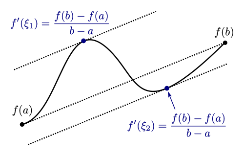
数学 において 、 平均値定理 ( ラグランジュの平均値定理 )は、大まかに言えば、2 つの端点間の平面 円弧 に対して、円弧の 接線がその端点を通る 割線 と平行になる点が少なくとも 1 つ存在することを述べています。これは 実解析 における最も重要な結果の 1 つです。この定理は 、区間の点における導関数に関する局所的な仮説から始めて、
区間 上の関数に関する記述を証明するために使用されます。
歴史 この定理 の逆正弦補間の 特殊なケースは、 インド の ケーララ天文数学学校の パラメシュヴァラ (1380–1460)が ゴーヴィンダスヴァーミ と バースカラII の注釈の中で初めて記述した 。 [1] この定理の限定された形式は、 1691年に ミシェル・ロールによって証明された。その結果は現在 ロールの定理 として知られており 、微積分の技術を使わずに多項式に対してのみ証明された。平均値定理の現代的な形式は、 1823年に オーギュスタン・ルイ・コーシーによって述べられ、証明された。 [2] この定理の多くのバリエーションがそれ以来証明されてきた。 [3] [4]
声明 関数は、 点 における導関数として 、 と の間の割線の傾きを得ます 。
ふ
{\displaystyle f}
1つの
{\displaystyle a}
b
{\displaystyle b}
ξ ∈ ( 1つの 、 b )
{\displaystyle \xi \in (a,b)}
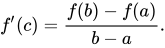
割線に平行な接線が複数存在する可能性もあります。 が閉区間 上の 連続関数 で 、 開区間 上 で 微分可能( ただし ) であると する 。 このとき、 には 次を 満たすものが存在する:
ふ : [ 1つの 、 b ] →
R
{\displaystyle f:[a,b]\to \mathbb {R} }
[ 1つの 、 b ]
{\displaystyle [a,b]}
( 1つの 、 b )
{\displaystyle (a,b)}
1つの < b
{\displaystyle a<b}
c
{\displaystyle c}
( 1つの 、 b )
{\displaystyle (a,b)}
ふ ′
( c ) =
ふ ( b ) − ふ ( 1つの )
b − 1つの
。
{\displaystyle f'(c)={\frac {f(b)-f(a)}{ba}}.}
平均値の定理は 、 を仮定して 上記の右辺がゼロになる
ロールの定理を一般化したものです。
ふ ( 1つの ) = ふ ( b )
{\displaystyle f(a)=f(b)}
平均値定理は、もう少し一般的な設定でも有効です。 が 上で 連続 であり 、極限の任意の に対して であると 仮定 する だけで十分です。
ふ : [ 1つの 、 b ] →
R
{\displaystyle f:[a,b]\to \mathbb {R} }
[ 1つの 、 b ]
{\displaystyle [a,b]}
x
{\displaystyle x}
( 1つの 、 b )
{\displaystyle (a,b)}
リム
h → 0
ふ ( x + h ) − ふ ( x )
h
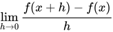
{\displaystyle \lim _{h\to 0}{\frac {f(x+h)-f(x)}{h}}}
は有限数として存在するか、 または または に等しい 。 が有限である場合、その極限は に等しい。 このバージョンの定理が適用される例として、 をマッピングする 実数値の 3 乗根 関数が挙げられます。この関数の 導関数は 原点で無限大に近づきます。
∞
{\displaystyle \infty}
− ∞
{\displaystyle -\infty}
ふ ′
( x )
{\displaystyle f'(x)}
x ↦
x
1
/
3
{\displaystyle x\mapsto x^{1/3}}
証拠 式は、 点 と を結ぶ線の 傾き を与えます 。これは のグラフの 弦 であり、 は 点 における曲線の接線の傾きを与えます 。したがって、平均値の定理によれば、滑らかな曲線の弦が与えられれば、弦の端点の間にある曲線上の点を見つけることができ、その点における曲線の接線は弦と平行になります。次の証明はこの考え方を示しています。
ふ ( b ) − ふ ( 1つの )
b − 1つの
{\textstyle {\frac {f(b)-f(a)}{ba}}}
( 1つの 、 ふ ( 1つの ) )
{\displaystyle (a,f(a))}
( b 、 ふ ( b ) )
{\displaystyle (b,f(b))}
ふ
{\displaystyle f}
ふ ′
( x )
{\displaystyle f'(x)}
( x 、 ふ ( x ) )
{\displaystyle (x,f(x))}
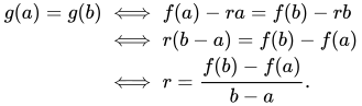
を定義します。 ここで は 定数です。 は で連続で で微分可能なので 、 についても同じことが言えます。ここで、 が ロールの定理 の条件を満たす ように を選びます 。つまり、
グ ( x ) = ふ ( x ) − r x
{\displaystyle g(x)=f(x)-rx}
r
{\displaystyle r}
ふ
{\displaystyle f}
[ 1つの 、 b ]
{\displaystyle [a,b]}
( 1つの 、 b )
{\displaystyle (a,b)}
グ
{\displaystyle g}
r
{\displaystyle r}
グ
{\displaystyle g}
グ ( 1つの ) = グ ( b )
⟺ ふ ( 1つの ) − r 1つの = ふ ( b ) − r b
⟺ r ( b − 1つの ) = ふ ( b ) − ふ ( 1つの )
⟺ r =
ふ ( b ) − ふ ( 1つの )
b − 1つの
。
{\displaystyle {\begin{aligned}g(a)=g(b)&\iff f(a)-ra=f(b)-rb\\&\iff r(ba)=f(b)-f(a)\\&\iff r={\frac {f(b)-f(a)}{ba}}.\end{aligned}}}
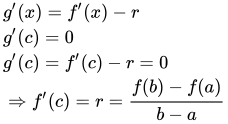
ロールの定理 によれば 、 は微分可能であり であるため、 において となる ものが存在し 、等式から次の式が導かれます 。
グ
{\displaystyle g}
グ ( 1つの ) = グ ( b )
{\displaystyle g(a)=g(b)}
c
{\displaystyle c}
( 1つの 、 b )
{\displaystyle (a,b)}
グ ′
( c ) = 0
{\displaystyle g'(c)=0}
グ ( x ) = ふ ( x ) − r x
{\displaystyle g(x)=f(x)-rx}
グ ′
( x ) =
ふ ′
( x ) − r
グ ′
( c ) = 0
グ ′
( c ) =
ふ ′
( c ) − r = 0
⇒
ふ ′
( c ) = r =
ふ ( b ) − ふ ( 1つの )
b − 1つの
{\displaystyle {\begin{aligned}&g'(x)=f'(x)-r\\&g'(c)=0\\&g'(c)=f'(c)-r=0\\&\Rightarrow f'(c)=r={\frac {f(b)-f(a)}{b-a}}\end{aligned}}}
意味合い 定理 1: は実数値関数であり、実数直線上の任意の区間で定義されていると 仮定します。 区間のすべての 内部点 で の の導関数が 存在し、ゼロである場合、 は 内部で
定数 です。
f
{\displaystyle f}
I
{\displaystyle I}
f
{\displaystyle f}
I
{\displaystyle I}
f
{\displaystyle f}
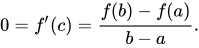
証明: 区間の あらゆる 内部点 におけるの導関数 が存在し、0であると仮定する。 を の任意の開区間とする 。平均値定理により、 には 次の点が存在する。
f
{\displaystyle f}
I
{\displaystyle I}
(
a
,
b
)
{\displaystyle (a,b)}
I
{\displaystyle I}
c
{\displaystyle c}
(
a
,
b
)
{\displaystyle (a,b)}
0
=
f
′
(
c
)
=
f
(
b
)
−
f
(
a
)
b
−
a
.
{\displaystyle 0=f'(c)={\frac {f(b)-f(a)}{b-a}}.}
これは、 を意味します 。したがって、 は の内部で定数であり 、連続性により 上で定数です 。(この結果の多変数バージョンについては以下を参照してください。)
f
(
a
)
=
f
(
b
)
{\displaystyle f(a)=f(b)}
f
{\displaystyle f}
I
{\displaystyle I}
I
{\displaystyle I}
備考:
区間 の端点では、の連続性のみが 必要であり、微分可能性は 必要ありません。 が 開区間 である場合、ある点での微分の存在は、この点での連続性を意味するため、連続性の仮定を述べる必要はありません。( 記事 「微分 」の 「連続性と微分可能性」 のセクションを参照してください 。)
f
{\displaystyle f}
I
{\displaystyle I}
I
{\displaystyle I}
の微分可能性は 片側微分可能性 に緩和することができ、その証明は 半微分可能性 に関する記事で与えられている 。
f
{\displaystyle f}
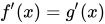
定理 2: これらの関数の定義域の 区間内の すべての に対してが定数である 場合、 は定数です 。
つまり、 は 上の定数です。
f
′
(
x
)
=
g
′
(
x
)
{\displaystyle f'(x)=g'(x)}
x
{\displaystyle x}
(
a
,
b
)
{\displaystyle (a,b)}
f
−
g
{\displaystyle f-g}
f
=
g
+
c
{\displaystyle f=g+c}
c
{\displaystyle c}
(
a
,
b
)
{\displaystyle (a,b)}
証明: とする と、 区間 上で となる ので、上記の定理 1 は が定数 または であることを示しています 。
F
(
x
)
=
f
(
x
)
−
g
(
x
)
{\displaystyle F(x)=f(x)-g(x)}
F
′
(
x
)
=
f
′
(
x
)
−
g
′
(
x
)
=
0
{\displaystyle F'(x)=f'(x)-g'(x)=0}
(
a
,
b
)
{\displaystyle (a,b)}
F
(
x
)
=
f
(
x
)
−
g
(
x
)
{\displaystyle F(x)=f(x)-g(x)}
c
{\displaystyle c}
f
=
g
+
c
{\displaystyle f=g+c}
定理 3: が区間 上の の原始積分である 場合、 上の の最も一般的な原始積分は であり 、 は 定数です。
F
{\displaystyle F}
f
{\displaystyle f}
I
{\displaystyle I}
f
{\displaystyle f}
I
{\displaystyle I}
F
(
x
)
+
c
{\displaystyle F(x)+c}
c
{\displaystyle c}
証明: 上記の定理 2 から直接導かれます。
コーシーの平均値定理 コーシーの平均値定理は、 拡張平均値定理 とも呼ばれ 、平均値定理の一般化である。 [6] これは、関数 とが 閉区間で連続であり 、開区間で微分可能である場合、 次のような
関数が存在することを述べている。
f
{\displaystyle f}
g
{\displaystyle g}
[
a
,
b
]
{\displaystyle [a,b]}
(
a
,
b
)
{\displaystyle (a,b)}
c
∈
(
a
,
b
)
{\displaystyle c\in (a,b)}
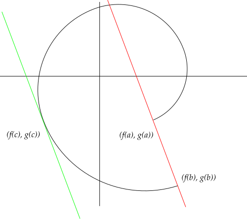
コーシーの定理の幾何学的意味
(
f
(
b
)
−
f
(
a
)
)
g
′
(
c
)
=
(
g
(
b
)
−
g
(
a
)
)
f
′
(
c
)
.
{\displaystyle (f(b)-f(a))g'(c)=(g(b)-g(a))f'(c).}
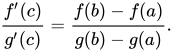
もちろん、 かつ の場合 、 これは次と同等です。
g
(
a
)
≠
g
(
b
)
{\displaystyle g(a)\neq g(b)}
g
′
(
c
)
≠
0
{\displaystyle g'(c)\neq 0}
f
′
(
c
)
g
′
(
c
)
=
f
(
b
)
−
f
(
a
)
g
(
b
)
−
g
(
a
)
.
{\displaystyle {\frac {f'(c)}{g'(c)}}={\frac {f(b)-f(a)}{g(b)-g(a)}}.}
幾何学的には、これは曲線 のグラフに何らかの 接線 があることを意味する [8]
{
[
a
,
b
]
→
R
2
t
↦
(
f
(
t
)
,
g
(
t
)
)
{\displaystyle {\begin{cases}[a,b]\to \mathbb {R} ^{2}\\t\mapsto (f(t),g(t))\end{cases}}}
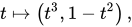
これは、点 と によって定義される直線に 平行 です。しかし、コーシーの定理は、と が異なる点 であるすべての場合にそのような接線が存在することを主張しているわけではありません。なぜなら、この定理は を伴うある値 、つまり、前述の曲線が 定常 となる 値に対して のみ満たされる可能性があるから です。そのような点では、曲線の接線はまったく定義されない可能性があります。この状況の例は、次で示される曲線です。
(
f
(
a
)
,
g
(
a
)
)
{\displaystyle (f(a),g(a))}
(
f
(
b
)
,
g
(
b
)
)
{\displaystyle (f(b),g(b))}
(
f
(
a
)
,
g
(
a
)
)
{\displaystyle (f(a),g(a))}
(
f
(
b
)
,
g
(
b
)
)
{\displaystyle (f(b),g(b))}
c
{\displaystyle c}
f
′
(
c
)
=
g
′
(
c
)
=
0
{\displaystyle f'(c)=g'(c)=0}
t
↦
(
t
3
,
1
−
t
2
)
,
{\displaystyle t\mapsto \left(t^{3},1-t^{2}\right),}
これは、区間 上で 点 から まで伸びます が、水平接線を持つことはありません。ただし、 に静止点 (実際には尖点 ) があります 。
[
−
1
,
1
]
{\displaystyle [-1,1]}
(
−
1
,
0
)
{\displaystyle (-1,0)}
(
1
,
0
)
{\displaystyle (1,0)}
t
=
0
{\displaystyle t=0}
コーシーの平均値定理は、ロピタルの定理 を証明するために使用できます 。平均値定理は、 の場合のコーシーの平均値定理の特殊なケースです 。
g
(
t
)
=
t
{\displaystyle g(t)=t}
証拠 コーシーの平均値定理の証明は、平均値定理の証明と同じ考えに基づいています。
と仮定する 。 を定義する。 ここで は となるように固定される 。すなわち
、
g
(
a
)
≠
g
(
b
)
{\displaystyle g(a)\neq g(b)}
h
(
x
)
=
f
(
x
)
−
r
g
(
x
)
{\displaystyle h(x)=f(x)-rg(x)}
r
{\displaystyle r}
h
(
a
)
=
h
(
b
)
{\displaystyle h(a)=h(b)}
h
(
a
)
=
h
(
b
)
⟺
f
(
a
)
−
r
g
(
a
)
=
f
(
b
)
−
r
g
(
b
)
⟺
r
(
g
(
b
)
−
g
(
a
)
)
=
f
(
b
)
−
f
(
a
)
⟺
r
=
f
(
b
)
−
f
(
a
)
g
(
b
)
−
g
(
a
)
.
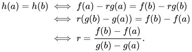
{\displaystyle {\begin{aligned}h(a)=h(b)&\iff f(a)-rg(a)=f(b)-rg(b)\\&\iff r(g(b)-g(a))=f(b)-f(a)\\&\iff r={\frac {f(b)-f(a)}{g(b)-g(a)}}.\end{aligned}}}
および は 上で連続で 上で微分可能な
ので 、 についても同じことが言えます 。 全体として、は ロールの定理 の条件を満たします。したがって、 には と なる が存在します 。 の定義を使用すると、次の式 が得られます。
f
{\displaystyle f}
g
{\displaystyle g}
[
a
,
b
]
{\displaystyle [a,b]}
(
a
,
b
)
{\displaystyle (a,b)}
h
{\displaystyle h}
h
{\displaystyle h}
c
{\displaystyle c}
(
a
,
b
)
{\displaystyle (a,b)}
h
′
(
c
)
=
0
{\displaystyle h'(c)=0}
h
{\displaystyle h}
0
=
h
′
(
c
)
=
f
′
(
c
)
−
r
g
′
(
c
)
=
f
′
(
c
)
−
(
f
(
b
)
−
f
(
a
)
g
(
b
)
−
g
(
a
)
)
g
′
(
c
)
,
{\displaystyle 0=h'(c)=f'(c)-rg'(c)=f'(c)-\left({\frac {f(b)-f(a)}{g(b)-g(a)}}\right)g'(c),}
そしてこうして
f
′
(
c
)
=
f
(
b
)
−
f
(
a
)
g
(
b
)
−
g
(
a
)
g
′
(
c
)
.
{\displaystyle f'(c)={\frac {f(b)-f(a)}{g(b)-g(a)}}g'(c).}
ならば 、 ロールの定理 を に適用すると、 に対して が 存在することがわかります 。 のこの選択を使用すると 、コーシーの平均値定理が(自明に)成り立ちます。
g
(
a
)
=
g
(
b
)
{\displaystyle g(a)=g(b)}
g
{\displaystyle g}
c
{\displaystyle c}
(
a
,
b
)
{\displaystyle (a,b)}
g
′
(
c
)
=
0
{\displaystyle g'(c)=0}
c
{\displaystyle c}
複数の変数における平均値定理 平均値の定理は、複数の変数の実関数に一般化されます。コツは、パラメータ化を使用して 1 つの変数の実関数を作成し、次に 1 変数の定理を適用することです。
を の開部分集合とし 、 を 微分可能関数とします。 間の線分が 内にあるように点を固定し 、 を定義します 。 は 1 変数の微分可能関数であるため、平均値定理により次のようになります。
G
{\displaystyle G}
R
n
{\displaystyle \mathbb {R} ^{n}}
f
:
G
→
R
{\displaystyle f:G\to \mathbb {R} }
x
,
y
∈
G
{\displaystyle x,y\in G}
x
,
y
{\displaystyle x,y}
G
{\displaystyle G}
g
(
t
)
=
f
(
(
1
−
t
)
x
+
t
y
)
{\displaystyle g(t)=f{\big (}(1-t)x+ty{\big )}}
g
{\displaystyle g}
g
(
1
)
−
g
(
0
)
=
g
′
(
c
)
{\displaystyle g(1)-g(0)=g'(c)}
0 から 1 の間の 値です。しかし、および なので 、明示的に 計算する と次のようになります。
c
{\displaystyle c}
g
(
1
)
=
f
(
y
)
{\displaystyle g(1)=f(y)}
g
(
0
)
=
f
(
x
)
{\displaystyle g(0)=f(x)}
g
′
(
c
)
{\displaystyle g'(c)}
f
(
y
)
−
f
(
x
)
=
∇
f
(
(
1
−
c
)
x
+
c
y
)
⋅
(
y
−
x
)
{\displaystyle f(y)-f(x)=\nabla f{\big (}(1-c)x+cy{\big )}\cdot (y-x)}
ここで、 は 勾配 と ドット 積 を表します 。これは、1 変数の定理の正確な類似です ( の場合は、 これは 1 変数の定理 です)。 コーシー・シュワルツの不等式 により、この式は次の推定値を与えます。
∇
{\displaystyle \nabla }
⋅
{\displaystyle \cdot }
n
=
1
{\displaystyle n=1}
|
f
(
y
)
−
f
(
x
)
|
≤
|
∇
f
(
(
1
−
c
)
x
+
c
y
)
|
|
y
−
x
|
.
{\displaystyle {\Bigl |}f(y)-f(x){\Bigr |}\leq {\Bigl |}\nabla f{\big (}(1-c)x+cy{\big )}{\Bigr |}\ {\Bigl |}y-x{\Bigr |}.}
特に、 が凸で の偏微分が 有界である場合、 は リプシッツ連続です (したがって 一様連続です )。
G
{\displaystyle G}
f
{\displaystyle f}
f
{\displaystyle f}
上記の応用として、 開集合 が連結で のすべての偏導関数が 0 であるとき、 は定数であることを証明します。ある点 を選び 、 とします。 すべての に対して であること を示します 。そのために とします 。すると は で閉じており 、空ではありません。 は開集合でもあります。すべての に対して 、
f
{\displaystyle f}
G
{\displaystyle G}
f
{\displaystyle f}
x
0
∈
G
{\displaystyle x_{0}\in G}
g
(
x
)
=
f
(
x
)
−
f
(
x
0
)
{\displaystyle g(x)=f(x)-f(x_{0})}
g
(
x
)
=
0
{\displaystyle g(x)=0}
x
∈
G
{\displaystyle x\in G}
E
=
{
x
∈
G
:
g
(
x
)
=
0
}
{\displaystyle E=\{x\in G:g(x)=0\}}
E
{\displaystyle E}
G
{\displaystyle G}
x
∈
E
{\displaystyle x\in E}
|
g
(
y
)
|
=
|
g
(
y
)
−
g
(
x
)
|
≤
(
0
)
|
y
−
x
|
=
0
{\displaystyle {\Big |}g(y){\Big |}={\Big |}g(y)-g(x){\Big |}\leq (0){\Big |}y-x{\Big |}=0}
を中心 とし に含まれる 任意の開球に対して となる 。 は 連結なので と結論付けられる 。
y
{\displaystyle y}
x
{\displaystyle x}
G
{\displaystyle G}
G
{\displaystyle G}
E
=
G
{\displaystyle E=G}
上記の議論は座標に依存しない方法で行われ、したがって、がバナッハ空間のサブセットである
場合に一般化されます。
G
{\displaystyle G}
ベクトル値関数の平均値定理 ベクトル値関数には平均値定理の正確な類似物はありません(下記参照)。しかし、1次元の場合に平均値定理が適用できる多くの状況に適用できる不等式があります:
平均値の不平等 ジャン・デュドネは、 その古典的論文 「現代解析学の基礎」 の中で平均値定理を捨てて平均不等式に置き換えた。これは、証明が構成的ではなく平均値を見つけることができず、応用では平均不等式のみが必要であるためである。 セルジュ・ラングは 解析学 I で 平均値定理を積分形式で即座に使用するが、この使用には導関数の連続性が必要である。 ヘンストック・カーツワイル積分を 使用すると、すべての導関数はヘンストック・カーツワイル積分可能であるため、導関数が連続しなければならないという追加の仮定なしに平均値定理を積分形式で持つことができる。
平均値の等式に類似するものがない理由は次の通りである。もし f : U → R m が微分可能関数(ただし U ⊂ R n は開関数)であり、 x + th , x , h ∈ R n , t ∈ [0, 1] が問題の線分( U の内部にある)であれば、上記のパラメータ化手順を f の各成分関数 f i ( i = 1, …, m ) に適用できる (上記の表記では y = x + h と設定)。そうすることで、次の式を満たす線分上の
点 x + t i hが見つかる。
f
i
(
x
+
h
)
−
f
i
(
x
)
=
∇
f
i
(
x
+
t
i
h
)
⋅
h
.
{\displaystyle f_{i}(x+h)-f_{i}(x)=\nabla f_{i}(x+t_{i}h)\cdot h.}
しかし、一般的には、線分上には
x + t * hを 満たす点が 1つも 存在しない。
f
i
(
x
+
h
)
−
f
i
(
x
)
=
∇
f
i
(
x
+
t
∗
h
)
⋅
h
.
{\displaystyle f_{i}(x+h)-f_{i}(x)=\nabla f_{i}(x+t^{*}h)\cdot h.}
すべてのi に対して 同時に と 定義します。たとえば、次のように定義します。
{
f
:
[
0
,
2
π
]
→
R
2
f
(
x
)
=
(
cos
(
x
)
,
sin
(
x
)
)
{\displaystyle {\begin{cases}f:[0,2\pi ]\to \mathbb {R} ^{2}\\f(x)=(\cos(x),\sin(x))\end{cases}}}
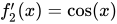
すると と なりますが 、 と は 上の範囲 では同時にゼロになることはありません 。
f
(
2
π
)
−
f
(
0
)
=
0
∈
R
2
{\displaystyle f(2\pi )-f(0)=\mathbf {0} \in \mathbb {R} ^{2}}
f
1
′
(
x
)
=
−
sin
(
x
)
{\displaystyle f_{1}'(x)=-\sin(x)}
f
2
′
(
x
)
=
cos
(
x
)
{\displaystyle f_{2}'(x)=\cos(x)}
x
{\displaystyle x}
[
0
,
2
π
]
{\displaystyle \left[0,2\pi \right]}
上記の定理は次のことを意味します。
実際、上記の記述は多くのアプリケーションに十分であり、次のように直接証明できます。(読みやすくするため に と書きます 。)
f
{\displaystyle f}
f
{\displaystyle {\textbf {f}}}
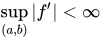
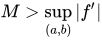
証拠 まず、が においても 微分可能であると仮定します 。が で 非有界である場合 、証明するものは何もありません。したがって、 と仮定します 。 を何らかの実数とします。 と
します。
を示したいと思います 。 の連続性により 、集合は 閉じています。 も のように空ではありません 。したがって、集合には 最大の要素 があります 。 の場合 、 であり 、 であるため、これで完了です。したがって、それ以外の場合を想定します。 の場合 、
f
{\displaystyle f}
a
{\displaystyle a}
f
′
{\displaystyle f'}
(
a
,
b
)
{\displaystyle (a,b)}
sup
(
a
,
b
)
|
f
′
|
<
∞
{\displaystyle \sup _{(a,b)}|f'|<\infty }
M
>
sup
(
a
,
b
)
|
f
′
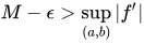
|
{\displaystyle M>\sup _{(a,b)}|f'|}
E
=
{
0
≤
t
≤
1
∣
|
f
(
a
+
t
(
b
−
a
)
)
−
f
(
a
)
|
≤
M
t
(
b
−
a
)
}
.
{\displaystyle E=\{0\leq t\leq 1\mid |f(a+t(b-a))-f(a)|\leq Mt(b-a)\}.}
1
∈
E
{\displaystyle 1\in E}
f
{\displaystyle f}
E
{\displaystyle E}
0
{\displaystyle 0}
E
{\displaystyle E}
s
{\displaystyle s}
s
=
1
{\displaystyle s=1}
1
∈
E
{\displaystyle 1\in E}
1
>
t
>
s
{\displaystyle 1>t>s}
|
f
(
a
+
t
(
b
−
a
)
)
−
f
(
a
)
|
≤
|
f
(
a
+
t
(
b
−
a
)
)
−
f
(
a
+
s
(
b
−
a
)
)
−
f
′
(
a
+
s
(
b
−
a
)
)
(
t
−
s
)
(
b
−
a
)
|
+
|
f
′
(
a
+
s
(
b
−
a
)
)
|
(
t
−
s
)
(
b
−
a
)
+
|
f
(
a
+
s
(
b
−
a
)
)
−
f
(
a
)
|
.
{\displaystyle {\begin{aligned}&|f(a+t(b-a))-f(a)|\\&\leq |f(a+t(b-a))-f(a+s(b-a))-f'(a+s(b-a))(t-s)(b-a)|+|f'(a+s(b-a))|(t-s)(b-a)\\&+|f(a+s(b-a))-f(a)|.\end{aligned}}}
を となるように 仮定します。 における の微分可能性により ( は 0 の場合もあることに注意)、 が に十分近い場合 、最初の項は です 。2 番目の項は です 。3 番目の項は です 。したがって、推定値を合計すると、 となり 、 の最大性と矛盾します 。したがって、となり 、これは次のことを意味します。
ϵ
>
0
{\displaystyle \epsilon >0}
M
−
ϵ
>
sup
(
a
,
b
)
|
f
′
|
{\displaystyle M-\epsilon >\sup _{(a,b)}|f'|}
f
{\displaystyle f}
a
+
s
(
b
−
a
)
{\displaystyle a+s(b-a)}
s
{\displaystyle s}
t
{\displaystyle t}
s
{\displaystyle s}
≤
ϵ
(
t
−
s
)
(
b
−
a
)
{\displaystyle \leq \epsilon (t-s)(b-a)}
≤
(
M
−
ϵ
)
(
t
−
s
)
(
b
−
a
)
{\displaystyle \leq (M-\epsilon )(t-s)(b-a)}
≤
M
s
(
b
−
a
)
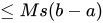
{\displaystyle \leq Ms(b-a)}
|
f
(
a
+
t
(
b
−
a
)
)
−
f
(
a
)
|
≤
t
M
|
b
−
a
|
{\displaystyle |f(a+t(b-a))-f(a)|\leq tM|b-a|}
s
{\displaystyle s}
1
=
s
∈
M
{\displaystyle 1=s\in M}
|
f
(
b
)
−
f
(
a
)
|
≤
M
(
b
−
a
)
.
{\displaystyle |f(b)-f(a)|\leq M(b-a).}
は任意なので 、これは次の主張を意味します。最後に、 が で微分可能でない場合 、 とし 、最初のケースを に 制限してに適用すると 、次のようになります。
M
{\displaystyle M}
f
{\displaystyle f}
a
{\displaystyle a}
a
′
∈
(
a
,
b
)
{\displaystyle a'\in (a,b)}
f
{\displaystyle f}
[
a
′
,
b
]
{\displaystyle [a',b]}
|
f
(
b
)
−
f
(
a
′
)
|
≤
(
b
−
a
′
)
sup
(
a
,
b
)
|
f
′
|
{\displaystyle |f(b)-f(a')|\leq (b-a')\sup _{(a,b)}|f'|}
なので 、これで 証明は終了です。
(
a
′
,
b
)
⊂
(
a
,
b
)
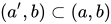
{\displaystyle (a',b)\subset (a,b)}
a
′
→
a
{\displaystyle a'\to a}
定理を適用できない場合 平均値定理の条件はすべて必要です。
f
(
x
)
{\displaystyle {\boldsymbol {f(x)}}}
は微分可能である
(
a
,
b
)
{\displaystyle {\boldsymbol {(a,b)}}}
f
(
x
)
{\displaystyle {\boldsymbol {f(x)}}}
継続中
[
a
,
b
]
{\displaystyle {\boldsymbol {[a,b]}}}
f
(
x
)
{\displaystyle {\boldsymbol {f(x)}}}
実数値である 上記の条件のいずれかが満たされない場合、平均値定理は一般に有効ではないため、適用できません。
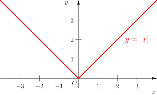
最初の条件の必要性は、[-1,1]上の関数が微分可能でないという反例によってわかります 。
f
(
x
)
=
|
x
|
{\displaystyle f(x)=|x|}
2 番目の条件の必要性は、関数がについては
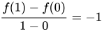
なので基準 1 を満たしているが 、 および について なので基準 2 を満たしていないという
反例によって確認できます
。 したがって 、 そのような関数 は存在しません。
f
(
x
)
=
{
1
,
at
x
=
0
0
,
if
x
∈
(
0
,
1
]
{\displaystyle f(x)={\begin{cases}1,&{\text{at }}x=0\\0,&{\text{if }}x\in (0,1]\end{cases}}}
f
′
(
x
)
=
0
{\displaystyle f'(x)=0}
(
0
,
1
)
{\displaystyle (0,1)}
f
(
1
)
−
f
(
0
)
1
−
0
=
−
1
{\displaystyle {\frac {f(1)-f(0)}{1-0}}=-1}
−
1
≠
0
=
f
′
(
x
)
{\displaystyle -1\neq 0=f'(x)}
x
∈
(
0
,
1
)
{\displaystyle x\in (0,1)}
c
{\displaystyle c}
微分可能関数が実数値ではなく複素数値である場合、定理は偽です。たとえば、 すべての実数 に対して である場合 、 ですが、
任意の実数 に対して
です 。
f
(
x
)
=
e
x
i
{\displaystyle f(x)=e^{xi}}
x
{\displaystyle x}
f
(
2
π
)
−
f
(
0
)
=
0
=
0
(
2
π
−
0
)
{\displaystyle f(2\pi )-f(0)=0=0(2\pi -0)}
f
′
(
x
)
≠
0
{\displaystyle f'(x)\neq 0}
x
{\displaystyle x}
定積分の平均値定理
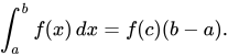
定積分における第一平均値定理 幾何学的には、f(c)を長方形の高さ、 b – aを幅と解釈すると、この長方形は aから b までの 曲線の下の領域と同じ面積を持つ [11] f : [ a , b ] → R を連続関数と する。すると、 ( a , b ) に次の式を
満たす c が存在する。
∫
a
b
f
(
x
)
d
x
=
f
(
c
)
(
b
−
a
)
.
{\displaystyle \int _{a}^{b}f(x)\,dx=f(c)(b-a).}
これは微積分学の基本定理 と微分に関する平均値定理 からすぐに導かれる。 [ a , b ]
における fの平均値は次のように定義されるので、
1
b
−
a
∫
a
b
f
(
x
)
d
x
,
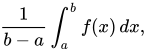
{\displaystyle {\frac {1}{b-a}}\int _{a}^{b}f(x)\,dx,}
この結論は、 fが ( a , b )のある c で平均値を達成する と解釈できる 。 [12]
一般に、 f : [ a , b ] → R が連続で、 g が[ a , b ]で符号が変化しない積分可能な関数である場合、 ( a , b ) に次の
c が 存在する。
∫
a
b
f
(
x
)
g
(
x
)
d
x
=
f
(
c
)
∫
a
b
g
(
x
)
d
x
.
{\displaystyle \int _{a}^{b}f(x)g(x)\,dx=f(c)\int _{a}^{b}g(x)\,dx.}
定積分における第二平均値定理 定積分に対する第二平均値定理 と呼ばれる、わずかに異なる定理がいくつか存在します 。よく見られるバージョンは次のとおりです。
が正の 単調減少 関数であり、が積分可能な関数である 場合、 ( a , b ]
に 数 xが存在し、
G
:
[
a
,
b
]
→
R
{\displaystyle G:[a,b]\to \mathbb {R} }
φ
:
[
a
,
b
]
→
R
{\displaystyle \varphi :[a,b]\to \mathbb {R} }
∫
a
b
G
(
t
)
φ
(
t
)
d
t
=
G
(
a
+
)
∫
a
x
φ
(
t
)
d
t
.
{\displaystyle \int _{a}^{b}G(t)\varphi (t)\,dt=G(a^{+})\int _{a}^{x}\varphi (t)\,dt.}
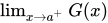
ここで は を表し、その存在は条件から導かれる。区間 ( a , b ]には b が含まれることが重要であることに注意してください 。この要件を持たない変形は次のようになります: [13]
G
(
a
+
)
{\displaystyle G(a^{+})}
lim
x
→
a
+
G
(
x
)
{\textstyle {\lim _{x\to a^{+}}G(x)}}
が単調 関数(必ずしも減少し正である必要はない) であり、が積分可能な関数である 場合、 ( a 、 b )
に 数 xが存在し、
G
:
[
a
,
b
]
→
R
{\displaystyle G:[a,b]\to \mathbb {R} }
φ
:
[
a
,
b
]
→
R
{\displaystyle \varphi :[a,b]\to \mathbb {R} }
∫
a
b
G
(
t
)
φ
(
t
)
d
t
=
G
(
a
+
)
∫
a
x
φ
(
t
)
d
t
+
G
(
b
−
)
∫
x
b
φ
(
t
)
d
t
.
{\displaystyle \int _{a}^{b}G(t)\varphi (t)\,dt=G(a^{+})\int _{a}^{x}\varphi (t)\,dt+G(b^{-})\int _{x}^{b}\varphi (t)\,dt.}
関数が 多次元ベクトルを返す場合、そのドメイン も多次元であっても、積分の MVT は真ではありません。
G
{\displaystyle G}
G
{\displaystyle G}
たとえば、 次元キューブ上で定義された次の 2 次元関数を考えます。
n
{\displaystyle n}
{
G
:
[
0
,
2
π
]
n
→
R
2
G
(
x
1
,
…
,
x
n
)
=
(
sin
(
x
1
+
⋯
+
x
n
)
,
cos
(
x
1
+
⋯
+
x
n
)
)
{\displaystyle {\begin{cases}G:[0,2\pi ]^{n}\to \mathbb {R} ^{2}\\G(x_{1},\dots ,x_{n})=\left(\sin(x_{1}+\cdots +x_{n}),\cos(x_{1}+\cdots +x_{n})\right)\end{cases}}}
すると、対称性により、その定義域における
の平均値は (0,0) であることが簡単にわかります。
G
{\displaystyle G}
∫
[
0
,
2
π
]
n
G
(
x
1
,
…
,
x
n
)
d
x
1
⋯
d
x
n
=
(
0
,
0
)
{\displaystyle \int _{[0,2\pi ]^{n}}G(x_{1},\dots ,x_{n})dx_{1}\cdots dx_{n}=(0,0)}
しかし、どこにでもある ので、そこに意味はありません 。
G
=
(
0
,
0
)
{\displaystyle G=(0,0)}
|
G
|
=
1
{\displaystyle |G|=1}
一般化
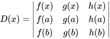
線形代数 およびは 上で連続な 上の 微分可能関数であると 仮定する 。定義
f
,
g
,
{\displaystyle f,g,}
h
{\displaystyle h}
(
a
,
b
)
{\displaystyle (a,b)}
[
a
,
b
]
{\displaystyle [a,b]}
D
(
x
)
=
|
f
(
x
)
g
(
x
)
h
(
x
)
f
(
a
)
g
(
a
)
h
(
a
)
f
(
b
)
g
(
b
)
h
(
b
)
|
{\displaystyle D(x)={\begin{vmatrix}f(x)&g(x)&h(x)\\f(a)&g(a)&h(a)\\f(b)&g(b)&h(b)\end{vmatrix}}}
となるようなもの が存在する 。
c
∈
(
a
,
b
)
{\displaystyle c\in (a,b)}
D
′
(
c
)
=
0
{\displaystyle D'(c)=0}
注意してください
D
′
(
x
)
=
|
f
′
(
x
)
g
′
(
x
)
h
′
(
x
)
f
(
a
)
g
(
a
)
h
(
a
)
f
(
b
)
g
(
b
)
h
(
b
)
|
{\displaystyle D'(x)={\begin{vmatrix}f'(x)&g'(x)&h'(x)\\f(a)&g(a)&h(a)\\f(b)&g(b)&h(b)\end{vmatrix}}}
を置けば、 コーシーの平均値定理 が 得られます 。 を置けば 、 ラグランジュの平均値定理 が 得られます 。
h
(
x
)
=
1
{\displaystyle h(x)=1}
h
(
x
)
=
1
{\displaystyle h(x)=1}
g
(
x
)
=
x
{\displaystyle g(x)=x}
一般化の証明は非常に簡単です。 および はそれぞれ 2 つの同一の 行 を持つ行列式で あるため、 です 。ロールの定理は、 となるようなが存在することを意味します 。
D
(
a
)
{\displaystyle D(a)}
D
(
b
)
{\displaystyle D(b)}
D
(
a
)
=
D
(
b
)
=
0
{\displaystyle D(a)=D(b)=0}
c
∈
(
a
,
b
)
{\displaystyle c\in (a,b)}
D
′
(
c
)
=
0
{\displaystyle D'(c)=0}
確率論 X と Yを 非負の ランダム変数 とし、E[ X ] < E[ Y ] < ∞ かつ (つまり、 通常の確率的順序 では Xは Y より小さい)とする。すると、 確率密度関数 を持つ 絶対連続な非負のランダム変数 Zが存在する。
X
≤
s
t
Y
{\displaystyle X\leq _{st}Y}
f
Z
(
x
)
=
Pr
(
Y
>
x
)
−
Pr
(
X
>
x
)
E
[
Y
]
−
E
[
X
]
,
x
⩾
0.
{\displaystyle f_{Z}(x)={\Pr(Y>x)-\Pr(X>x) \over {\rm {E}}[Y]-{\rm {E}}[X]}\,,\qquad x\geqslant 0.}
g を 測定可能 かつ 微分可能な関数 と し 、E[ g ( X )], E[ g ( Y )] < ∞ とし、その導関数 g′ をすべての y ≥ x ≥ 0 に対して区間 [ x , y ]上で 測定可能かつ リーマン積分可能 とする。このとき、E[ g′ ( Z )] は有限であり、 [14]
E
[
g
(
Y
)
]
−
E
[
g
(
X
)
]
=
E
[
g
′
(
Z
)
]
[
E
(
Y
)
−
E
(
X
)
]
.
{\displaystyle {\rm {E}}[g(Y)]-{\rm {E}}[g(X)]={\rm {E}}[g'(Z)]\,[{\rm {E}}(Y)-{\rm {E}}(X)].}
複雑な分析 上で述べたように、この定理は微分可能な複素数値関数には当てはまらない。その代わりに、この定理の一般化は次のように述べられる: [15]
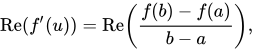
f : Ω → C を 開凸集合Ω上の 正則関数 とし 、 a と bをΩ内の異なる点とする。すると、 aから b への 線分の内部に点 u 、 vが 存在し 、
Re
(
f
′
(
u
)
)
=
Re
(
f
(
b
)
−
f
(
a
)
b
−
a
)
,
{\displaystyle \operatorname {Re} (f'(u))=\operatorname {Re} \left({\frac {f(b)-f(a)}{b-a}}\right),}
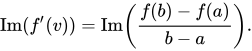
Im
(
f
′
(
v
)
)
=
Im
(
f
(
b
)
−
f
(
a
)
b
−
a
)
.
{\displaystyle \operatorname {Im} (f'(v))=\operatorname {Im} \left({\frac {f(b)-f(a)}{b-a}}\right).}
ここで、Re() は複素数値関数の実数部、Im() は虚数部です。
参照
注記
^ JJ O'ConnorとEF Robertson (2000). Paramesvara、 MacTutor数学史アーカイブ 。 ^ アダム・ベセニエイ。 「平均値定理の歴史的展開」 (PDF) 。 ^ Lozada-Cruz, German (2020-10-02). 「コーシーの平均値定理のいくつかのバリエーション」. 国際科学技術数学教育ジャーナル . 51 (7): 1155–1163. Bibcode :2020IJMES..51.1155L. doi :10.1080/0020739X.2019.1703150. ISSN 0020-739X. S2CID 213335491. ^ Sahoo, Prasanna. (1998). 平均値定理と関数方程式. Riedel, T. (Thomas), 1962-. シンガポール: World Scientific. ISBN 981-02-3544-5 . OCLC 40951137. ^ W., Weisstein, Eric. 「拡張平均値定理」. mathworld.wolfram.com . 2018年10月8日 閲覧 。 {{cite web}}: CS1 maint: multiple names: authors list (link)^ 「コーシーの平均値定理」 。Math24 。 2018年10月8日 閲覧。 ^ Hörmander 2015、定理1.1.1。およびそれに続く注釈。 ^ 「Mathwords: 積分の平均値定理」 www.mathwords.com 。 ^ Michael Comenetz (2002). 微積分学: 要素 . World Scientific. p. 159. ISBN 978-981-02-4904-5 。 ^ Hobson, EW (1909). 「積分法の第二平均値定理について」. Proc. London Math. Soc. S2–7 (1): 14–23. Bibcode :1909PLMS...27...14H. doi :10.1112/plms/s2-7.1.14. MR 1575669. ^ Di Crescenzo, A. (1999). 「平均値定理の確率的類似物と信頼性理論への応用」 J. Appl. Probab. 36 (3): 706–719. doi :10.1239/jap/1032374628. JSTOR 3215435. S2CID 250351233. ^ 1 J.-Cl. Evard、F. Jafari、「複雑なロールの定理」、American Mathematical Monthly、第99巻、第9号、(1992年11月)、pp. 858-861。
参考文献 ルディン、ウォルター(1976)。数学的解析 の 原理 。オークランド:McGraw-Hill Publishing Company。ISBN 978-0-07-085613-4 。 ヘルマンダー、ラース (2015)、 線形偏微分演算子の解析I:分布理論とフーリエ解析 、数学の古典(第2版)、シュプリンガー、 ISBN 9783642614972
外部リンク



![{\displaystyle f:[a,b]\to \mathbb {R} }](https://wikimedia.org/api/rest_v1/media/math/render/svg/b592d102ccd1ba134d401c5b3ea177baaba3ffac)
![{\displaystyle [a,b]}](https://wikimedia.org/api/rest_v1/media/math/render/svg/9c4b788fc5c637e26ee98b45f89a5c08c85f7935)





















![{\displaystyle {\begin{cases}[a,b]\to \mathbb {R} ^{2}\\t\mapsto (f(t),g(t))\end{cases}}}](https://wikimedia.org/api/rest_v1/media/math/render/svg/035d912ebe2e72e28cf8922a39d1b07ee8afe321)



![{\displaystyle [-1,1]}](https://wikimedia.org/api/rest_v1/media/math/render/svg/51e3b7f14a6f70e614728c583409a0b9a8b9de01)
























![{\displaystyle \mathbf {f} :[a,b]\to \mathbb {R} ^{k}}](https://wikimedia.org/api/rest_v1/media/math/render/svg/80ca56b7a396adc60daac6924b7d1ab63f91d3a9)











![{\displaystyle {\begin{cases}f:[0,2\pi ]\to \mathbb {R} ^{2}\\f(x)=(\cos(x),\sin(x))\end{cases}}}](https://wikimedia.org/api/rest_v1/media/math/render/svg/537a6776144419319a90c743f3bfa85384551b8e)


![{\displaystyle \left[0,2\pi \right]}](https://wikimedia.org/api/rest_v1/media/math/render/svg/ecbccc3195ac7ed59d31ec366dbd75739b85e1d3)
![{\displaystyle {\textbf {f}}:[a,b]\to \mathbb {R} ^{k}}](https://wikimedia.org/api/rest_v1/media/math/render/svg/e00619b1c9ca88ab6f218f7c42e472895b00c8c6)

















![{\displaystyle [a',b]}](https://wikimedia.org/api/rest_v1/media/math/render/svg/a2199a20ce14a38267ad303f042837644e8feb46)



![{\displaystyle {\boldsymbol {[a,b]}}}](https://wikimedia.org/api/rest_v1/media/math/render/svg/be8b220f66f725e30a237bcebb00bc3459c2471f)

![{\displaystyle f(x)={\begin{cases}1,&{\text{at }}x=0\\0,&{\text{if }}x\in (0,1]\end{cases}}}](https://wikimedia.org/api/rest_v1/media/math/render/svg/0cb6e79196b3cfc68f23749dc33e5c9d7c878cfe)









![{\displaystyle G:[a,b]\to \mathbb {R} }](https://wikimedia.org/api/rest_v1/media/math/render/svg/7b03d8b7acec0b034f6d4d9e1b3a538e1a8cf8cc)
![{\displaystyle \varphi :[a,b]\to \mathbb {R} }](https://wikimedia.org/api/rest_v1/media/math/render/svg/4e34d6980745c5c3dfc05229082eb4f4c017a5c0)




![{\displaystyle {\begin{cases}G:[0,2\pi ]^{n}\to \mathbb {R} ^{2}\\G(x_{1},\dots ,x_{n})=\left(\sin(x_{1}+\cdots +x_{n}),\cos(x_{1}+\cdots +x_{n})\right)\end{cases}}}](https://wikimedia.org/api/rest_v1/media/math/render/svg/313681274f21ab3d719858b7eee2f8fed7307df7)
![{\displaystyle \int _{[0,2\pi ]^{n}}G(x_{1},\dots ,x_{n})dx_{1}\cdots dx_{n}=(0,0)}](https://wikimedia.org/api/rest_v1/media/math/render/svg/800b9da34869b8de54b9e67e50211354ff1230c9)






![{\displaystyle f_{Z}(x)={\Pr(Y>x)-\Pr(X>x) \over {\rm {E}}[Y]-{\rm {E}}[X]}\,,\qquad x\geqslant 0.}](https://wikimedia.org/api/rest_v1/media/math/render/svg/98380bb043d37ca11885348245ab1f1e05019170)
![{\displaystyle {\rm {E}}[g(Y)]-{\rm {E}}[g(X)]={\rm {E}}[g'(Z)]\,[{\rm {E}}(Y)-{\rm {E}}(X)].}](https://wikimedia.org/api/rest_v1/media/math/render/svg/4d3a485925f91f6271a2201cc6cc46b4d5d381f6)