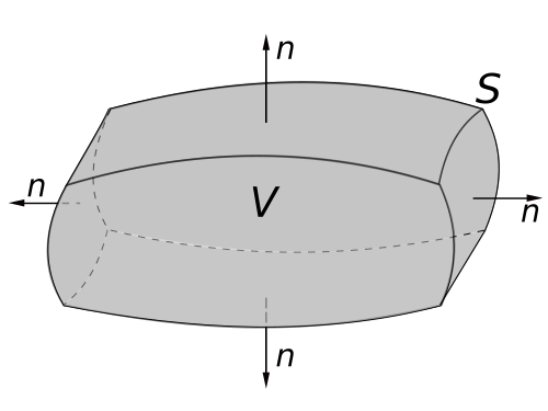
液体の流れを用いた説明 ベクトル場は 、気体や液体などの流体の 速度 場を例に説明されることが多い。移動する液体は、各点で速度(速さと方向)を持ち、これはベクトル で表すことができるため、任意の瞬間の液体の速度はベクトル場を形成する。液体の体積を囲む液体の内部にある閉じた表面Sを考える。任意の時点で体積から流出する液体の 流量 は、この表面を通過する流体の体積流量、つまり表面上の速度の面積分に等しい。
非圧縮性流体を仮定すると、閉じた体積内の液体の量は一定です。体積内に供給源や吸収源がない場合、 S から流出する液体の流量はゼロになります。液体が移動している場合、表面S 上のいくつかの点で体積内に流入し、他の点で体積外に流出する可能性がありますが、任意の瞬間における流入量と流出量は等しいため、体積から流出する液体の正味流量はゼロになります。
しかし、閉じた表面の内側に液体の供給源 (例えば、液体を導入するパイプ)がある場合、追加された液体は周囲の液体に圧力をかけ、あらゆる方向に外向きの流れを引き起こします。これにより、表面Sを通る正味の外向きの流れが生じます。S を 通る外向きの流れは、パイプからS に流入する液体の体積流量に等しくなります。同様に、 Sの内側に シンク または排水口(例えば、液体を排出するパイプ)がある場合、液体の外部圧力により、液体全体に排水口の位置に向かって内向きの速度が生じます。表面S を通る内向きの液体の体積流量は、シンクによって除去される液体の流量に等しくなります。
S 内に液体の供給源と排出口が複数ある場合、表面を通過する流量は、供給源によって加えられる液体の体積流量を合計し、排出口によって排出される液体の流量を差し引くことによって計算できます。供給源または排出口を通過する液体の体積流量(排出口を通過する流量には負の符号が付けられます)は、パイプの開口部での速度場の発散 に等しいので、 S で囲まれた体積全体にわたって液体の発散を合計(積分)すると、S を通過する流量の体積流量に等しくなります。これが発散定理です。[ 2 ]
発散定理は、すべてのシンクとソースの総体積、つまり発散の体積積分が、体積の境界を横切る正味の流れに等しいことを示すあらゆる保存則に用いられます。 [ 3 ]
発散定理は、体積V が別々の部分に分割された場合、元の体積からのフラックス は各構成要素体積からのフラックスの代数和に等しいという事実から導かれる。[ 6 ] [ 7 ]
体積を2つの部分体積に分割した図。右側では、2つの部分体積を分離して、異なる表面からの流出量を示している。 図を参照してください。閉じた境界のある体積V は、表面S 3 (緑色)によって 2 つの体積 V 1 V 2 V i Φ( V i ) は、その 2 つの面を通過するフラックスの合計に等しいので、2 つの部分からのフラックスの合計は次のようになります。
Φ ( V 1 ) + Φ ( V 2 ) = Φ 1 + Φ 31 + Φ 2 + Φ 32 {\displaystyle \Phi (V_{\text{1}})+\Phi (V_{\text{2}})=\Phi _{\text{1}}+\Phi _{\text{31}}+\Phi _{\text{2}}+\Phi _{\text{32}}} ここで、Φ 1 とΦ 2は表面 S 1 S 2 Φ 31 は体積 1 からS 3 Φ 32は体積 2 から S 3 S 3 が両方の体積の表面の一部であるということです。法線ベクトル の「外向き」方向n ^ {\displaystyle \mathbf {\hat {n}} } 各体積に対して逆なので、 S 3
Φ 31 = ∬ S 3 F ⋅ n ^ d S = − ∬ S 3 F ⋅ ( − n ^ ) d S = − Φ 32 {\displaystyle \Phi _{\text{31}}=\iint _{S_{3}}\mathbf {F} \cdot \mathbf {\hat {n}} \;\mathrm {d} S=-\iint _{S_{3}}\mathbf {F} \cdot (-\mathbf {\hat {n}} )\;\mathrm {d} S=-\ファイ _{\text{32}}} したがって:
Φ ( V 1 ) + Φ ( V 2 ) = Φ 1 + Φ 2 {\displaystyle \Phi (V_{\text{1}})+\Phi (V_{\text{2}})=\Phi _{\text{1}}+\Phi _{\text{2}}} 曲面S 1 S 2 S であるため
Φ ( V 1 ) + Φ ( V 2 ) = Φ ( V ) {\displaystyle \ファイ (V_{\text{1}})+\ファイ (V_{\text{2}})=\ファイ (V)}
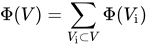
体積は任意の数のサブボリュームに分割でき、V からのフラックスは各サブボリュームからのフラックスの合計に等しくなります。これは、緑色の 表面を通過するフラックスが合計で相殺されるためです。(b)では、体積がわずかに離れて表示されており、各緑色の分割が隣接する2つの体積の境界の一部であることを示しています。 この原理は、図に示すように、任意の数の部分に分割された体積に適用されます。[ 7 ] 各内部分割(緑色の表面) (灰色)
Φ ( V ) = ∑ V 私 ⊂ V Φ ( V 私 ) {\displaystyle \Phi (V)=\sum _{V_{\text{i}}\subset V}\Phi (V_{\text{i}})}
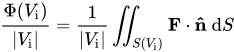
体積がより小さな部分に分割されるにつれて、流量の比率はΦ ( V 私 ) {\displaystyle \Phi (V_{\text{i}})} | V 私 | {\displaystyle |V_{\text{i}}|} div F {\displaystyle \operatorname {div} \mathbf {F} } 各体積からのフラックスΦ は、ベクトル場F ( x )
∬ S ( V ) F ⋅ n ^ d S = ∑ V 私 ⊂ V ∬ S ( V 私 ) F ⋅ n ^ d S {\displaystyle \iint _{S(V)}\mathbf {F} \cdot \mathbf {\hat {n}} \;\mathrm {d} S=\sum _{V_{\text{i}}\subset V}\iint _{S(V_{\text{i}})}\mathbf {F} \cdot \mathbf {\hat {n}} \;\mathrm {d} S} 目標は、元の体積を無限に多くの微小体積に分割することです。体積がますます小さな部分に分割されるにつれて、右側の表面積分、各部分体積からのフラックスは、表面積S ( V i )がゼロに近づくため、ゼロに近づきます。しかし、発散 の定義から、フラックスと体積の比は、Φ ( V 私 ) | V 私 | = 1 | V 私 | ∬ S ( V 私 ) F ⋅ n ^ d S {\displaystyle {\frac {\Phi (V_{\text{i}})}{|V_{\text{i}}|}}={\frac {1}{|V_{\text{i}}|}}\iint _{S(V_{\text{i}})}\mathbf {F} \cdot \mathbf {\hat {n}} \;\mathrm {d} S} 発散 div Fに近づきます。 [ 7 ]
∬ S ( V ) F ⋅ n ^ d S = ∑ V 私 ⊂ V ( 1 | V 私 | ∬ S ( V 私 ) F ⋅ n ^ d S ) | V 私 | {\displaystyle \iint _{S(V)}\mathbf {F} \cdot \mathbf {\hat {n}} \;\mathrm {d} S=\sum _{V_{\text{i}}\subset V}\left({\frac {1}{|V_{\text{i}}|}}\iint _{S(V_{\text{i}})}\mathbf {F} \cdot \mathbf {\hat {n}} \;\mathrm {d} S\right)|V_{\text{i}}|} ベクトル場F ( x )極限 においても上記の和は成り立つ。
∬ S ( V ) F ⋅ n ^ d S = リム | V 私 | → 0 ∑ V 私 ⊂ V ( 1 | V 私 | ∬ S ( V 私 ) F ⋅ n ^ d S ) | V 私 | {\displaystyle \iint _{S(V)}\mathbf {F} \cdot \mathbf {\hat {n}} \;\mathrm {d} S=\lim _{|V_{\text{i}}|\to 0}\sum _{V_{\text{i}}\subset V}\left({\frac {1}{|V_{\text{i}}|}}\iint _{S(V_{\text{i}})}\mathbf {F} \cdot \mathbf {\hat {n}} \;\mathrm {d} S\right)|V_{\text{i}}|} として| V 私 | {\displaystyle |V_{\text{i}}|} dV V に関する体積積分となる。
∬ S ( V ) F ⋅ n ^ d S = ∭ V div F d V {\displaystyle \;\iint _{S(V)}\mathbf {F} \cdot \mathbf {\hat {n}} \;\mathrm {d} S=\iiint _{V}\operatorname {div} \mathbf {F} \;\mathrm {d} V\;}
この導出は座標に依存しないため、発散は使用する座標に依存しないことが示される。
証明
ユークリッド空間の有界開部分集合の場合 私たちは以下のことを証明します。
定理の証明。 [ 8 ]
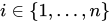
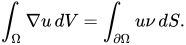
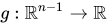
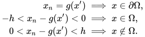
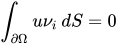
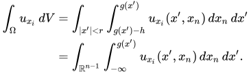
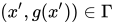
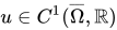
最初のステップは、次のケースに還元することです。u ∈ C c 1 ( R n ) {\displaystyle u\in C_{c}^{1}(\mathbb {R} ^{n})} ϕ ∈ C c ∞ ( O ) {\displaystyle \phi \in C_{c}^{\infty }(O)} ϕ = 1 {\displaystyle \phi =1} Ω ¯ {\displaystyle {\overline {\Omega }}} ϕ u ∈ C c 1 ( O ) ⊂ C c 1 ( R n ) {\displaystyle \phi u\in C_{c}^{1}(O)\subset C_{c}^{1}(\mathbb {R} ^{n})} ϕ u = u {\displaystyle \phi u=u} Ω ¯ {\displaystyle {\overline {\Omega }}} ϕ u {\displaystyle \phi u} u ∈ C c 1 ( R n ) {\displaystyle u\in C_{c}^{1}(\mathbb {R} ^{n})} させてx 0 ∈ ∂ Ω {\displaystyle x_{0}\in \partial \Omega } Ω ¯ {\displaystyle {\overline {\Omega }}} C 1 {\displaystyle C^{1}} U {\displaystyle U} x 0 {\displaystyle x_{0}} R n {\displaystyle \mathbb {R} ^{n}} ∂ Ω ∩ U {\displaystyle \partial \Omega \cap U} C 1 {\displaystyle C^{1}} Ω ∩ U {\displaystyle \Omega \cap U} Ω {\displaystyle \Omega } r > 0 {\displaystyle r>0} h > 0 {\displaystyle h>0} C 1 {\displaystyle C^{1}} g : R n − 1 → R {\displaystyle g:\mathbb {R} ^{n-1}\to \mathbb {R} } x ′ = ( x 1 、 … 、 x n − 1 ) 、 {\displaystyle x'=(x_{1},\dots ,x_{n-1}),} U = { x ∈ R n : | x ′ | < r そして | x n − g ( x ′ ) | < h } {\displaystyle U=\{x\in \mathbb {R} ^{n}:|x'|<r{\text{ and }}|x_{n}-g(x')|<h\}} x ∈ U {\displaystyle x\in U} x n = g ( x ′ ) ⟹ x ∈ ∂ Ω 、 − h < x n − g ( x ′ ) < 0 ⟹ x ∈ Ω 、 0 < x n − g ( x ′ ) < h ⟹ x ∉ Ω 。 {\displaystyle {\begin{aligned}x_{n}=g(x')&\implies x\in \partial \Omega ,\\-h<x_{n}-g(x')<0&\implies x\in \Omega ,\\0<x_{n}-g(x')<h&\implies x\notin \Omega .\\\end{aligned}}} ∂ Ω {\displaystyle \partial \Omega } ∂ Ω {\displaystyle \partial \Omega } U 1 、 … 、 U N {\displaystyle U_{1},\dots ,U_{N}} { Ω 、 U 1 、 … 、 U N } {\displaystyle \{\Omega ,U_{1},\dots ,U_{N}\}} Ω ¯ = Ω ∪ ∂ Ω {\displaystyle {\overline {\Omega }}=\Omega \cup \partial \Omega } C ∞ {\displaystyle C^{\infty }} この被覆に従属する統一性の分割の場合 、以下のいずれかの場合に定理を証明すれば十分である。u {\displaystyle u} サポート を備えていますΩ {\displaystyle \Omega } u {\displaystyle u} U j {\displaystyle U_{j}} u {\displaystyle u} Ω {\displaystyle \Omega } 私 ∈ { 1 、 … 、 n } {\displaystyle i\in \{1,\dots ,n\}} ∫ Ω u x 私 d V = ∫ R n u x 私 d V = ∫ R n − 1 ∫ − ∞ ∞ u x 私 ( x ) d x 私 d x ′ = 0 {\displaystyle \int _{\Omega }u_{x_{i}}\,dV=\int _{\mathbb {R} ^{n}}u_{x_{i}}\,dV=\int _{\mathbb {R} ^{n-1}}\int _{-\infty }^{\infty }u_{x_{i}}(x)\,dx_{i}\,dx'=0} ∫ ∂ Ω u ν 私 d S = 0 {\displaystyle \int _{\partial \Omega }u\nu _{i}\,dS=0} u {\displaystyle u} ∂ Ω {\displaystyle \partial \Omega } u {\displaystyle u} Ω {\displaystyle \Omega } u {\displaystyle u} U j {\displaystyle U_{j}} では、u {\displaystyle u} U j {\displaystyle U_{j}} U = U j {\displaystyle U=U_{j}} U {\displaystyle U} Ω {\displaystyle \Omega } u ( x ) = 0 {\displaystyle u(x)=0} | x ′ | ≥ r {\displaystyle |x'|\geq r} | x n − g ( x ′ ) | ≥ h {\displaystyle |x_{n}-g(x')|\geq h} 私 ∈ { 1 、 … 、 n } {\displaystyle i\in \{1,\dots ,n\}} ∫ Ω u x 私 d V = ∫ | x ′ | < r ∫ g ( x ′ ) − h g ( x ′ ) u x 私 ( x ′ 、 x n ) d x n d x ′ = ∫ R n − 1 ∫ − ∞ g ( x ′ ) u x 私 ( x ′ 、 x n ) d x n d x ′ 。 {\displaystyle {\begin{aligned}\int _{\Omega }u_{x_{i}}\,dV&=\int _{|x'|<r}\int _{g(x')-h}^{g(x')}u_{x_{i}}(x',x_{n})\,dx_{n}\,dx'\\&=\int _{\mathbb {R} ^{n-1}}\int _{-\infty }^{g(x')}u_{x_{i}}(x',x_{n})\,dx_{n}\,dx'.\end{aligned}}} 私 = n {\displaystyle i=n} ∫ R n − 1 ∫ − ∞ g ( x ′ ) u x n ( x ′ 、 x n ) d x n d x ′ = ∫ R n − 1 u ( x ′ 、 g ( x ′ ) ) d x ′ 。 {\displaystyle \int _{\mathbb {R} ^{n-1}}\int _{-\infty }^{g(x')}u_{x_{n}}(x',x_{n})\,dx_{n}\,dx'=\int _{\mathbb {R} ^{n-1}}u(x',g(x'))\,dx'.} 私 ∈ { 1 、 … 、 n − 1 } {\displaystyle i\in \{1,\dots ,n-1\}} ∫ R n − 1 ∫ − ∞ g ( x ′ ) u x 私 ( x ′ 、 x n ) d x n d x ′ = ∫ R n − 1 ∫ − ∞ 0 u x 私 ( x ′ 、 g ( x ′ ) + s ) d s d x ′ {\displaystyle \int _{\mathbb {R} ^{n-1}}\int _{-\infty }^{g(x')}u_{x_{i}}(x',x_{n})\,dx_{n}\,dx'=\int _{\mathbb {R} ^{n-1}}\int _{-\infty }^{0}u_{x_{i}}(x',g(x')+s)\,ds\,dx'} v : R n → R {\displaystyle v:\mathbb {R} ^{n}\to \mathbb {R} } v ( x ′ 、 s ) = u ( x ′ 、 g ( x ′ ) + s ) {\displaystyle v(x',s)=u(x',g(x')+s)} v x 私 ( x ′ 、 s ) = u x 私 ( x ′ 、 g ( x ′ ) + s ) + u x n ( x ′ 、 g ( x ′ ) + s ) g x 私 ( x ′ ) 。 {\displaystyle v_{x_{i}}(x',s)=u_{x_{i}}(x',g(x')+s)+u_{x_{n}}(x',g(x')+s)g_{x_{i}}(x').} v {\displaystyle v} d x 私 {\displaystyle dx_{i}} ∫ R n − 1 ∫ − ∞ 0 v x 私 ( x ′ 、 s ) d s d x ′ = 0. {\displaystyle \int _{\mathbb {R} ^{n-1}}\int _{-\infty }^{0}v_{x_{i}}(x',s)\,ds\,dx'=0.} ∫ R n − 1 ∫ − ∞ 0 u x 私 ( x ′ 、 g ( x ′ ) + s ) d s d x ′ = ∫ R n − 1 ∫ − ∞ 0 − u x n ( x ′ 、 g ( x ′ ) + s ) g x 私 ( x ′ ) d s d x ′ = ∫ R n − 1 − u ( x ′ 、 g ( x ′ ) ) g x 私 ( x ′ ) d x ′ 。 {\displaystyle {\begin{aligned}\int _{\mathbb {R} ^{n-1}}\int _{-\infty }^{0}u_{x_{i}}(x',g(x')+s)\,ds\,dx'&=\int _{\mathbb {R} ^{n-1}}\int _{-\infty }^{0}-u_{x_{n}}(x',g(x')+s)g_{x_{i}}(x')\,ds\,dx'\\&=\int _{\mathbb {R} ^{n-1}}-u(x',g(x'))g_{x_{i}}(x')\,dx'.\end{aligned}}} ∇ u = ( u x 1 、 … 、 u x n ) {\displaystyle \nabla u=(u_{x_{1}},\dots ,u_{x_{n}})} ∫ Ω ∇ u d V = ∫ R n − 1 ∫ − ∞ g ( x ′ ) ∇ u d V = ∫ R n − 1 u ( x ′ 、 g ( x ′ ) ) ( − ∇ g ( x ′ ) 、 1 ) d x ′ 。 {\displaystyle \int _{\Omega }\nabla u\,dV=\int _{\mathbb {R} ^{n-1}}\int _{-\infty }^{g(x')}\nabla u\,dV=\int _{\mathbb {R} ^{n-1}}u(x',g(x'))(-\nabla g(x'),1)\,dx'.} Γ {\displaystyle \Gamma } g {\displaystyle g} ( x ′ 、 g ( x ′ ) ) ∈ Γ {\displaystyle (x',g(x'))\in \Gamma } ν ( x ′ 、 g ( x ′ ) ) = 1 1 + | ∇ g ( x ′ ) | 2 ( − ∇ g ( x ′ ) 、 1 ) {\displaystyle \nu (x',g(x'))={\frac {1}{\sqrt {1+|\nabla g(x')|^{2}}}}(-\nabla g(x'),1)} d S {\displaystyle dS} d S = 1 + | ∇ g ( x ′ ) | 2 d x ′ {\textstyle dS={\sqrt {1+|\nabla g(x')|^{2}}}\,dx'} ∫ Ω ∇ u d V = ∫ ∂ Ω u ν d S 。 {\displaystyle \int _{\Omega }\nabla u\,dV=\int _{\partial \Omega }u\nu \,dS.}
境界を持つコンパクトなリーマン多様体の場合 私たちは以下のことを証明します。
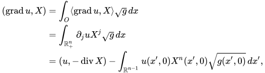
定理の証明。 [ 9 ] u {\displaystyle u} X {\displaystyle X} O ⊂ Ω ¯ {\displaystyle O\subset {\overline {\Omega }}} ∂ Ω {\displaystyle \partial \Omega } O {\displaystyle O} R n {\displaystyle \mathbb {R} ^{n}} ( 卒業生 u 、 X ) = ∫ O ⟨ 卒業生 u 、 X ⟩ g d x = ∫ O ∂ j u X j g d x = − ∫ O u ∂ j ( g X j ) d x = − ∫ O u 1 g ∂ j ( g X j ) g d x = ( u 、 − 1 g ∂ j ( g X j ) ) = ( u 、 − div X ) 。 {\displaystyle {\begin{aligned}(\operatorname {grad} u,X)&=\int _{O}\langle \operatorname {grad} u,X\rangle {\sqrt {g}}\,dx\\&=\int _{O}\partial _{j}uX^{j}{\sqrt {g}}\,dx\\[5pt]&=-\int _{O}u\partial _{j}\left({\sqrt {g}}X^{j}\right)\,dx\\[5pt]&=-\int _{O}u{\frac {1}{\sqrt {g}}}\partial _{j}\left({\sqrt {g}}X^{j}\right){\sqrt {g}}\,dx\\[5pt]&=\left(u,-{\frac {1}{\sqrt {g}}}\partial _{j}\left({\sqrt {g}}X^{j}\right)\right)\\[5pt]&=(u,-\operatorname {div} X).\end{aligned}}} − div {\displaystyle -\operatorname {div} } 卒業生 {\displaystyle \operatorname {grad} } O {\displaystyle O} ∂ Ω {\displaystyle \partial \Omega } O {\displaystyle O} R + n = { x ∈ R n : x n ≥ 0 } {\displaystyle \mathbb {R} _{+}^{n}=\{x\in \mathbb {R} ^{n}:x_{n}\geq 0\}} u {\displaystyle u} X {\displaystyle X} R + n {\displaystyle \mathbb {R} _{+}^{n}} ( 卒業生 u 、 X ) = ∫ O ⟨ 卒業生 u 、 X ⟩ g d x = ∫ R + n ∂ j u X j g d x = ( u 、 − div X ) − ∫ R n − 1 u ( x ′ 、 0 ) X n ( x ′ 、 0 ) g ( x ′ 、 0 ) d x ′ 、 {\displaystyle {\begin{aligned}(\operatorname {grad} u,X)&=\int _{O}\langle \operatorname {grad} u,X\rangle {\sqrt {g}}\,dx\\&=\int _{\mathbb {R} _{+}^{n}}\partial _{j}uX^{j}{\sqrt {g}}\,dx\\&=(u,-\operatorname {div} X)-\int _{\mathbb {R} ^{n-1}}u(x',0)X^{n}(x',0){\sqrt {g(x',0)}}\,dx',\end{aligned}}} d x ′ = d x 1 ⋯ d x n − 1 {\displaystyle dx'=dx_{1}\cdots dx_{n-1}} ベクトル場の直線化定理 の変形により、O {\displaystyle O} ∂ ∂ x n {\displaystyle {\frac {\partial }{\partial x_{n}}}} − N {\displaystyle -N} ∂ Ω {\displaystyle \partial \Omega } g ( x ′ 、 0 ) d x ′ = g ∂ Ω ( x ′ ) d x ′ = d S {\displaystyle {\sqrt {g(x',0)}}\,dx'={\sqrt {g_{\partial \Omega }(x')}}\,dx'=dS} ∂ Ω {\displaystyle \partial \Omega } ( 卒業生 u 、 X ) = ( u 、 − div X ) + ∫ ∂ Ω u ⟨ X 、 N ⟩ d S 。 {\displaystyle (\operatorname {grad} u,X)=(u,-\operatorname {div} X)+\int _{\partial \Omega }u\langle X,N\rangle \,dS.}
系 発散定理のF を ベクトル恒等式 を参照)。[ 10 ]
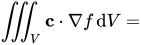
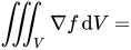
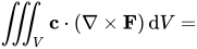
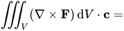
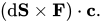
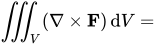
とF → F g {\displaystyle \mathbf {F} \rightarrow \mathbf {F} g} g とベクトル場F ∭ V [ F ⋅ ( ∇ g ) + g ( ∇ ⋅ F ) ] d V = {\displaystyle \iiint _{V}\left[\mathbf {F} \cdot \left(\nabla g\right)+g\left(\nabla \cdot \mathbf {F} \right)\right]\mathrm {d} V=} S {\displaystyle \scriptstyle S} g F ⋅ n d S 。 {\displaystyle g\mathbf {F} \cdot \mathbf {n} \,\mathrm {d} S.} この特殊なケースはF = ∇ f {\displaystyle \mathbf {F} =\nabla f} グリーンの恒等式 の基礎となる。 とF → F × G {\displaystyle \mathbf {F} \rightarrow \mathbf {F} \times \mathbf {G} } F G × {\displaystyle \times } ∭ V ∇ ⋅ ( F × G ) d V = ∭ V [ G ⋅ ( ∇ × F ) − F ⋅ ( ∇ × G ) ] d V = {\displaystyle \iiint _{V}\nabla \cdot \left(\mathbf {F} \times \mathbf {G} \right)\mathrm {d} V=\iiint _{V}\left[\mathbf {G} \cdot \left(\nabla \times \mathbf {F} \right)-\mathbf {F} \cdot \left(\nabla \times \mathbf {G} \right)\right]\,\mathrm {d} V=} S {\displaystyle \scriptstyle S} ( F × G ) ⋅ n d S 。 {\displaystyle (\mathbf {F} \times \mathbf {G} )\cdot \mathbf {n} \,\mathrm {d} S.} とF → F ⋅ G {\displaystyle \mathbf {F} \rightarrow \mathbf {F} \cdot \mathbf {G} } F G ⋅ {\displaystyle \cdot } は内積 を表します。 ∭ V ∇ ( F ⋅ G ) d V = ∭ V [ ( ∇ G ) ⋅ F + ( ∇ F ) ⋅ G ] d V = {\displaystyle \iiint _{V}\nabla \left(\mathbf {F} \cdot \mathbf {G} \right)\mathrm {d} V=\iiint _{V}\left[\left(\nabla \mathbf {G} \right)\cdot \mathbf {F} +\left(\nabla \mathbf {F} \right)\cdot \mathbf {G} \right]\,\mathrm {d} V=} S {\displaystyle \scriptstyle S} ( F ⋅ G ) n d S 。 {\displaystyle (\mathbf {F} \cdot \mathbf {G} )\mathbf {n} \,\mathrm {d} S.} とF → f c {\displaystyle \mathbf {F} \rightarrow f\mathbf {c} } f c の場合:[ 11 ] ∭ V c ⋅ ∇ f d V = {\displaystyle \iiint _{V}\mathbf {c} \cdot \nabla f\,\mathrm {d} V=} S {\displaystyle \scriptstyle S} ( c f ) ⋅ n d S − ∭ V f ( ∇ ⋅ c ) d V 。 {\displaystyle (\mathbf {c} f)\cdot \mathbf {n} \,\mathrm {d} S-\iiint _{V}f(\nabla \cdot \mathbf {c} )\,\mathrm {d} V.} 右辺の最後の項は定数の場合に消滅するc {\displaystyle \mathbf {c} } c {\displaystyle \mathbf {c} } ∭ V ∇ f d V = {\displaystyle \iiint _{V}\nabla f\,\mathrm {d} V=} S {\displaystyle \scriptstyle S} f n d S 。 {\displaystyle f\mathbf {n} \,\mathrm {d} S.} とF → c × F {\displaystyle \mathbf {F} \rightarrow \mathbf {c} \times \mathbf {F} } F c の場合:[ 11 ] ∭ V c ⋅ ( ∇ × F ) d V = {\displaystyle \iiint _{V}\mathbf {c} \cdot (\nabla \times \mathbf {F} )\,\mathrm {d} V=} S {\displaystyle \scriptstyle S} ( F × c ) ⋅ n d S 。 {\displaystyle (\mathbf {F} \times \mathbf {c} )\cdot \mathbf {n} \,\mathrm {d} S.} 右辺の三重積 を並べ替え、積分の定数ベクトルを取り出すことにより、 ∭ V ( ∇ × F ) d V ⋅ c = {\displaystyle \iiint _{V}(\nabla \times \mathbf {F} )\,\mathrm {d} V\cdot \mathbf {c} =} S {\displaystyle \scriptstyle S} ( d S × F ) ⋅ c 。 {\displaystyle (\mathrm {d} \mathbf {S} \times \mathbf {F} )\cdot \mathbf {c} .} したがって、 ∭ V ( ∇ × F ) d V = {\displaystyle \iiint _{V}(\nabla \times \mathbf {F} )\,\mathrm {d} V=} S {\displaystyle \scriptstyle S} n × F d S 。 {\displaystyle \mathbf {n} \times \mathbf {F} \,\mathrm {d} S.}
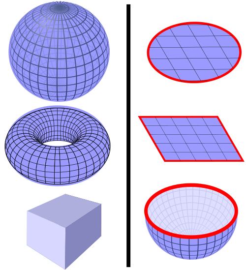
例 図に示された例に対応するベクトル場。ベクトルは球面の内側または外側を向いている場合があります。 発散定理は、左側の図にあるような、体積を完全に囲む閉曲面を通過する流量を計算するために使用できます。しかし、右側の図にあるような境界を持つ曲面を通過する流量を計算するために直接使用することはでき ません 。(曲面は青色、境界は赤色で示されています。) 評価したいとしましょう
S {\displaystyle \scriptstyle S} F ⋅ n d S 、 {\displaystyle \mathbf {F} \cdot \mathbf {n} \,\mathrm {d} S,} ここで、S は次のように定義される単位球 である。
S = { ( x 、 y 、 z ) ∈ R 3 : x 2 + y 2 + z 2 = 1 } 、 {\displaystyle S=\left\{(x,y,z)\in \mathbb {R} ^{3}\ :\ x^{2}+y^{2}+z^{2}=1\right\},} F ベクトル場 である
F = 2 x 私 + y 2 j + z 2 k 。 {\displaystyle \mathbf {F} =2x\mathbf {i} +y^{2}\mathbf {j} +z^{2}\mathbf {k} .} この積分を直接計算するのは非常に難しいが、発散定理を用いることで結果の導出を簡略化できる。なぜなら、発散定理によれば、この積分は次のように表されるからである。
∭ W ( ∇ ⋅ F ) d V = 2 ∭ W ( 1 + y + z ) d V = 2 ∭ W d V + 2 ∭ W y d V + 2 ∭ W z d V 、 {\displaystyle {\begin{aligned}\iiint _{W}(\nabla \cdot \mathbf {F} )\,\mathrm {d} V&=2\iiint _{W}\left(1+y+z\right)\ \mathrm {d} V\\&=2\iiint _{W}\mathrm {d} V+2\iiint _{W}y\,\mathrm {d} V+2\iiint _{W}z\,\mathrm {d} V,\end{aligned}}} ここでWは 単位球 である。
W = { ( x 、 y 、 z ) ∈ R 3 : x 2 + y 2 + z 2 ≤ 1 } 。 {\displaystyle W=\left\{(x,y,z)\in \mathbb {R} ^{3}\ :\ x^{2}+y^{2}+z^{2}\leq 1\right\}.} 関数yは W の一方の半球では正、もう一方の半球では負となるため、等しく反対の方向に、W全体にわたる y の積分値はゼロになります 。z についても同様です。
∭ W y d V = ∭ W z d V = 0. {\displaystyle \iiint _{W}y\,\mathrm {d} V=\iiint _{W}z\,\mathrm {d} V=0.} したがって、
S {\displaystyle \scriptstyle S} F ⋅ n d S = 2 ∭ W d V = 8 π 3 、 {\displaystyle \mathbf {F} \cdot \mathbf {n} \,\mathrm {d} S=2\iiint _{W}\,dV={\frac {8\pi }{3}},} なぜなら、単位球W の 体積 は4π / 3 だから です
アプリケーション
発散定理の結果として、多くの物理法則は微分形式(ある量が別の量の発散として表される)と積分形式(閉曲面を通過するある量の流量が別の量に等しい)の両方で記述することができる。その例として、ガウスの法則 (静電気学 )、ガウスの磁気法則 、ガウスの重力法則 が挙げられる。
計算例
例1 領域に対する発散定理の平面版を検証するR {\displaystyle R}
R = { ( x 、 y ) ∈ R 2 : x 2 + y 2 ≤ 1 } 、 {\displaystyle R=\left\{(x,y)\in \mathbb {R} ^{2}\ :\ x^{2}+y^{2}\leq 1\right\},} そしてベクトル場:
F ( x 、 y ) = 2 y 私 + 5 x j 。 {\displaystyle \mathbf {F} (x,y)=2y\mathbf {i} +5x\mathbf {j} .} 境界R {\displaystyle R} C {\displaystyle C}
x = コス ( s ) 、 y = 罪 ( s ) {\displaystyle x=\cos(s),\quad y=\sin(s)} そのため0 ≤ s ≤ 2 π {\displaystyle 0\leq s\leq 2\pi } s {\displaystyle s} s = 0 {\displaystyle s=0} P {\displaystyle P} C {\displaystyle C} C {\displaystyle C}
C ( s ) = コス ( s ) 私 + 罪 ( s ) j 。 {\displaystyle C(s)=\cos(s)\mathbf {i} +\sin(s)\mathbf {j} .} ある時点でP {\displaystyle P} C {\displaystyle C}
P = ( コス ( s ) 、 罪 ( s ) ) ⇒ F = 2 罪 ( s ) 私 + 5 コス ( s ) j 。 {\displaystyle P=(\cos(s),\,\sin(s))\,\Rightarrow \,\mathbf {F} =2\sin(s)\mathbf {i} +5\cos(s)\mathbf {j} .} したがって、
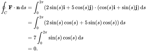
∮ C F ⋅ n d s = ∫ 0 2 π ( 2 罪 ( s ) 私 + 5 コス ( s ) j ) ⋅ ( コス ( s ) 私 + 罪 ( s ) j ) d s = ∫ 0 2 π ( 2 罪 ( s ) コス ( s ) + 5 罪 ( s ) コス ( s ) ) d s = 7 ∫ 0 2 π 罪 ( s ) コス ( s ) d s = 0. {\displaystyle {\begin{aligned}\oint _{C}\mathbf {F} \cdot \mathbf {n} \,\mathrm {d} s&=\int _{0}^{2\pi }(2\sin(s)\mathbf {i} +5\cos(s)\mathbf {j} )\cdot (\cos(s)\mathbf {i} +\sin(s)\mathbf {j} )\,\mathrm {d} s\\&=\int _{0}^{2\pi }(2\sin(s)\cos(s)+5\sin(s)\cos(s))\,\mathrm {d} s\\&=7\int _{0}^{2\pi }\sin(s)\cos(s)\,\mathrm {d} s\\&=0.\end{aligned}}} なぜならM = R e ( F ) = 2 y {\displaystyle M={\mathfrak {Re}}(\mathbf {F} )=2y} ∂ M ∂ x = 0 {\displaystyle {\frac {\partial M}{\partial x}}=0} N = 私 m ( F ) = 5 x {\displaystyle N={\mathfrak {Im}}(\mathbf {F} )=5x} ∂ N ∂ y = 0 {\displaystyle {\frac {\partial N}{\partial y}}=0}
∬ R ∇ ⋅ F d A = ∬ R ( ∂ M ∂ x + ∂ N ∂ y ) d A = 0. {\displaystyle \iint _{R}\,\mathbf {\nabla } \cdot \mathbf {F} \,\mathrm {d} A=\iint _{R}\left({\frac {\partial M}{\partial x}}+{\frac {\partial N}{\partial y}}\right)\,\mathrm {d} A=0.}
例2 次のベクトル場 のフラックスを評価したいとしましょう。F = 2 x 2 私 + 2 y 2 j + 2 z 2 k {\displaystyle \mathbf {F} =2x^{2}{\textbf {i}}+2y^{2}{\textbf {j}}+2z^{2}{\textbf {k}}}
{ 0 ≤ x ≤ 3 } 、 { − 2 ≤ y ≤ 2 } 、 { 0 ≤ z ≤ 2 π } {\displaystyle \left\{0\leq x\leq 3\right\},\left\{-2\leq y\leq 2\right\},\left\{0\leq z\leq 2\pi \right\}} 発散定理により、
∭ V ( ∇ ⋅ F ) d V = {\displaystyle \iiint _{V}\left(\mathbf {\nabla } \cdot \mathbf {F} \right)\mathrm {d} V=} S {\displaystyle \scriptstyle S} ( F ⋅ n ) d S 。 {\displaystyle (\mathbf {F} \cdot \mathbf {n} )\,\mathrm {d} S.} 次に、F {\displaystyle {\textbf {F}}} F {\displaystyle \mathbf {F} } F {\displaystyle {\textbf {F}}} ∇ ⋅ F = ( ∂ ∂ x 私 + ∂ ∂ y j + ∂ ∂ z k ) ⋅ F {\textstyle \nabla \cdot {\textbf {F}}=\left({\frac {\partial }{\partial x}}{\textbf {i}}+{\frac {\partial }{\partial y}}{\textbf {j}}+{\frac {\partial }{\partial z}}{\textbf {k}}\right)\cdot {\textbf {F}}}
したがって、次のフラックス積分を立てることができます。私 = {\displaystyle I=} S {\displaystyle {\scriptstyle S}} F ⋅ n d S 、 {\displaystyle \mathbf {F} \cdot \mathbf {n} \,\mathrm {d} S,}
私 = ∭ V ∇ ⋅ F d V = ∭ V ( ∂ F x ∂ x + ∂ F y ∂ y + ∂ F z ∂ z ) d V = ∭ V ( 4 x + 4 y + 4 z ) d V = ∫ 0 3 ∫ − 2 2 ∫ 0 2 π ( 4 x + 4 y + 4 z ) d V {\displaystyle {\begin{aligned}I&=\iiint _{V}\nabla \cdot \mathbf {F} \,\mathrm {d} V\\[6pt]&=\iiint _{V}\left({\frac {\partial \mathbf {F_{x}} }{\partial x}}+{\frac {\partial \mathbf {F_{y}} }{\partial y}}+{\frac {\partial \mathbf {F_{z}} }{\partial z}}\right)\mathrm {d} V\\[6pt]&=\iiint _{V}(4x+4y+4z)\,\mathrm {d} V\\[6pt]&=\int _{0}^{3}\int _{-2}^{2}\int _{0}^{2\pi }(4x+4y+4z)\,\mathrm {d} V\end{aligned}}} 積分式ができたので、これを計算してみましょう。
∫ 0 3 ∫ − 2 2 ∫ 0 2 π ( 4 x + 4 y + 4 z ) d V = ∫ − 2 2 ∫ 0 2 π ( 12 y + 12 z + 18 ) d y d z = ∫ 0 2 π 24 ( 2 z + 3 ) d z = 48 π ( 2 π + 3 ) {\displaystyle {\begin{aligned}\int _{0}^{3}\int _{-2}^{2}\int _{0}^{2\pi }(4x+4y+4z)\,\mathrm {d} V&=\int _{-2}^{2}\int _{0}^{2\pi }(12y+12z+18)\,\mathrm {d} y\,\mathrm {d} z\\[6pt]&=\int _{0}^{2\pi }24(2z+3)\,\mathrm {d} z\\[6pt]&=48\pi (2\pi +3)\end{aligned}}}
一般化
多次元 一般化されたストークスの定理 を用いると、領域U上のベクトル場 F n 次元体積積分を、U の境界上のF の( n − 1) 次元面積積分と等しくすることができる。
∫ ⋯ ∫ U ⏟ n ∇ ⋅ F d V = ∮ ⋯ ∮ ∂ U ⏟ n − 1 F ⋅ n d S {\displaystyle \underbrace {\int \cdots \int _{U}} _{n}\nabla \cdot \mathbf {F} \,\mathrm {d} V=\underbrace {\oint \cdots \oint _{\partial U}} _{n-1}\mathbf {F} \cdot \mathbf {n} \,\mathrm {d} S} この方程式は発散定理としても知られています。
n = 2グリーンの定理 と同等です。
n = 1微積分学の基本定理の パート 2 に帰着します。
参考文献 ↑ Katz, Victor J. (1979). 「ストークスの定理の歴史」. Mathematics Magazine . 52 (3): 146– 156. doi : 10.2307/2690275 . JSTOR 2690275 . アンダーソン、マーロウ(2009)『誰があなた に イプシロンを与えたのか?:そして数学史のその他の物語』 アメリカ数学協会、78-79ページ に 。ISBN 978-0-88385-569-0 。↑ RG Lerner ; GL Trigg (1994). 物理学百科事典 (第2 版). VHC. ISBN 978-3-527-26954-9 。↑ バイロン、フレデリック; フラー、ロバート (1992)、 『古典物理学と量子物理学の数学』 、ドーバー出版、 22 ページ 、 ISBN 978-0-486-67164-2 ↑ Wiley, C. Ray Jr. 『Advanced Engineering Mathematics, 3rd Ed 』McGraw-Hill、pp. 372–373 。 ↑ クレイジグ、アーウィン;クレイジグ、ハーバート;ノーミントン、エドワード J. (2011). 高度工学数学 (第10 版). ジョン・ワイリー・アンド・サンズ. pp. 453–456 . ISBN 978-0-470-45836-5 。↑ ベンフォード、フランク A. (2007 年 5 月)。 「ベクトル解析に関するノート」 (PDF) 。 数学 105: 多変数微積分コースの教材 。ウィリアムズ大学スティーブン ミラー教授のウェブページ 。2022 年 3 月 14 日に 取得。 1 2 3 パーセル、エドワード M.、デイビッド J. モリン (2013)。 電気と磁気 。 ケンブリッジ大学出版局。56–58 ページ 。ISBN 978-1-107-01402-2 。↑ Alt, Hans Wilhelm (2016). "線形関数解析". Universitext . ロンドン: Springer London. pp. 259–261 , 270–272 . doi : 10.1007/978-1-4471-7280-2 . ISBN 978-1-4471-7279-6 ISSN 0172-5939 ↑ Taylor, Michael E. (2011). "偏微分方程式 I". 応用数理科学 第 115巻. ニューヨーク、NY: Springer New York. pp. 178–179 . doi : 10.1007/978-1-4419-7055-8 . ISBN 978-1-4419-7054-1 ISSN 0066-5452 ↑ MRシュピーゲル。 S. リプシュッツ; D. スペルマン (2009)。 ベクトル解析 。シャウムの概要(第 2 版)。アメリカ:マグロウヒル。 ISBN 978-0-07-161545-7 。1 2 数学の世界 1 2 C.B.パーカー(1994)。 マグロウヒル物理学百科事典 ( 第2 版)。マグロウヒル。ISBN 978-0-07-051400-3 。1 2 カッツ、ヴィクター (2009)。「第22章:ベクトル解析」。 『数学史入門』。アディソン ・ ウェスリー。808-809 頁 。ISBN 978-0-321-38700-4 。↑ 音に関する 1762 年の論文で、ラグランジュは発散定理の特殊なケースを扱っています: Lagrange (1762) "Nouvelles recherches sur la Nature et la propagation duson" (音の性質と伝播に関する新しい研究)、 Miscellanea Taurinensia (別名: Mélanges de Turin )、 2 : 11 – 172。この記事は次のように再版されます。「自然と伝播の新研究」 、JA Serret 編、 Oeuvres de Lagrange 、(パリ、フランス: Gauthier-Villars、1867)、vol. 1、151~316ページ。 263 ~ 265 ページで、ラグランジュは部分積分を使用して三重積分を二重積分に変換します。 ↑ CF Gauss (1813)「Theoria Attractis corporum sphaeroicorum ellipticorum homogeneorum methodo nova tractata」、Commentationes societatis regiae scientiarium Gottingensis Recentiores 、 2 : 355–378;ガウスは定理の特殊な場合を考えました。彼の記事の 4、5、6 ページを参照してください。 1 2 3 Katz, Victor (1979 年 5 月). 「ストークスの定理の歴史」. Mathematics Magazine . 52 (3): 146–156 . doi : 10.1080/0025570X.1979.11976770 . JSTOR 2690275 . ↑ ミハイル・オストラグラツキーは1826年にパリ科学アカデミーに発散定理の証明を発表しましたが、その論文はアカデミーによって出版されませんでした。彼はロシアのサンクトペテルブルクに戻り、1828年から1829年にかけてフランスで行った研究をサンクトペテルブルク科学アカデミーで発表し、アカデミーは1831年にその論文を要約版として出版しました。 彼が1826年2月13日にパリ・アカデミーで発表した発散定理の証明「Démonstration d'un théorème du calcul intégral」(積分計算における定理の証明)は、1965年に彼の別の論文とともにロシア語に翻訳された。参照:Юшкевич А.П.(ユシュケヴィチ AP)およびАнтропова В.И。 (アントロポフ VI) (1965) 「Неопубликованные работы М.В. Остроградского」(MV Ostrogradskii の未発表作品)、Историко-математические исследования (Istoriko-Matematicheskie Isledovaniya / 歴史数学研究)、16 : 49–96; 「Остроградский М.В. Доказательство одной теоремы интегрального исчисления」というタイトルのセクションを参照してください。 Ostragradsky MV 積分微積分における定理の証明)。 M. Ostrogradsky (発表: 1828 年 11 月 5 日; 出版: 1831 年) 「Première note sur la théorie de la Chaleur」 (熱理論に関する最初のメモ) Mémoires de l'Académie impériale des Sciences de St. Pétersbourg 、シリーズ 6、1 : 129–133。発散定理の彼の証明の短縮版については、130 ~ 131 ページを参照してください。 Victor J. Katz (1979 年 5 月) 「ストークスの定理の歴史」、Wayback Machine に 2015 年 4 月 2 日に アーカイブ済み、Mathematics Magazine 、52 (3): 146–156 doi : 10.1080/0025570X.1979.11976770 ; オストラグラツキーによる発散定理の証明については、147–148 ページを参照。 ↑ ジョージ・グリーン著『電気と磁気の理論への数学的解析の応用に関するエッセイ』 (英国ノッティンガム:T. Wheelhouse、1838年)。「発散定理」の一形式が 10~12ページに掲載されている。 ↑ 発散定理の何らかの形を用いた初期の研究者には、以下のような人物がいる。 ポアソン (発表:1824年2月2日、出版:1826年)「磁気理論に関する覚書」(Mémoire sur la théorie du magnétisme)、フランス学士院科学アカデミー紀要 、5 :247–338;294–296ページで、ポアソンは体積積分(量Qを評価するために用いられる)を面積積分に変換している。この変換を行うために、ポアソンは発散定理を証明する際に用いられるのと同じ手順に従っている。Frédéric Sarrus (1828) 「Mémoire sur les oscillations des corps flottans」(浮遊体の振動に関する回想録)、Annales de mathématiques pures et appliquées (Nismes)、19 : 185–211。 ↑ KF ライリー、MP ホブソン、SJ ベンス (2010)。 物理学および工学のための数学的手法 。ケンブリッジ大学出版局 。ISBN 978-0-521-86153-3 。↑ 例えば、 JA Wheeler、C. Misner、KS Thorne (1973) 『重力』 WH Freeman & Co.、pp. 85–86 、§3.5を参照 。ISBN 978-0-7167-0344-0 。R.ペンローズ (2007)。 『現実への道』 。ヴィンテージブックス 。ISBN 978-0-679-77631-4 。 
























































![{\displaystyle {\begin{aligned}(\operatorname {grad} u,X)&=\int _{O}\langle \operatorname {grad} u,X\rangle {\sqrt {g}}\,dx\\&=\int _{O}\partial _{j}uX^{j}{\sqrt {g}}\,dx\\[5pt]&=-\int _{O}u\partial _{j}\left({\sqrt {g}}X^{j}\right)\,dx\\[5pt]&=-\int _{O}u{\frac {1}{\sqrt {g}}}\partial _{j}\left({\sqrt {g}}X^{j}\right){\sqrt {g}}\,dx\\[5pt]&=\left(u,-{\frac {1}{\sqrt {g}}}\partial _{j}\left({\sqrt {g}}X^{j}\right)\right)\\[5pt]&=(u,-\operatorname {div} X).\end{aligned}}}](https://wikimedia.org/api/rest_v1/media/math/render/svg/20ccee48b8434b5164d70506bda12f4a5f185660)









![{\displaystyle \iiint _{V}\left[\mathbf {F} \cdot \left(\nabla g\right)+g\left(\nabla \cdot \mathbf {F} \right)\right]\mathrm {d} V=}](https://wikimedia.org/api/rest_v1/media/math/render/svg/4e2423d13911c2504aaa900e167209926272cf9e)


![{\displaystyle \iiint _{V}\nabla \cdot \left(\mathbf {F} \times \mathbf {G} \right)\mathrm {d} V=\iiint _{V}\left[\mathbf {G} \cdot \left(\nabla \times \mathbf {F} \right)-\mathbf {F} \cdot \left(\nabla \times \mathbf {G} \right)\right]\,\mathrm {d} V=}](https://wikimedia.org/api/rest_v1/media/math/render/svg/7545c1e2a215463f96180aa6566fc932cbf2fafb)


![{\displaystyle \iiint _{V}\nabla \left(\mathbf {F} \cdot \mathbf {G} \right)\mathrm {d} V=\iiint _{V}\left[\left(\nabla \mathbf {G} \right)\cdot \mathbf {F} +\left(\nabla \mathbf {F} \right)\cdot \mathbf {G} \right]\,\mathrm {d} V=}](https://wikimedia.org/api/rest_v1/media/math/render/svg/3d8e82e763d252526e5c5cb4518b3615d250dc81)




































![{\displaystyle {\begin{aligned}I&=\iiint _{V}\nabla \cdot \mathbf {F} \,\mathrm {d} V\\[6pt]&=\iiint _{V}\left({\frac {\partial \mathbf {F_{x}} }{\partial x}}+{\frac {\partial \mathbf {F_{y}} }{\partial y}}+{\frac {\partial \mathbf {F_{z}} }{\partial z}}\right)\mathrm {d} V\\[6pt]&=\iiint _{V}(4x+4y+4z)\,\mathrm {d} V\\[6pt]&=\int _{0}^{3}\int _{-2}^{2}\int _{0}^{2\pi }(4x+4y+4z)\,\mathrm {d} V\end{aligned}}}](https://wikimedia.org/api/rest_v1/media/math/render/svg/d474d797d9611bde7396b5ad3c477fc3954e40fb)
![{\displaystyle {\begin{aligned}\int _{0}^{3}\int _{-2}^{2}\int _{0}^{2\pi }(4x+4y+4z)\,\mathrm {d} V&=\int _{-2}^{2}\int _{0}^{2\pi }(12y+12z+18)\,\mathrm {d} y\,\mathrm {d} z\\[6pt]&=\int _{0}^{2\pi }24(2z+3)\,\mathrm {d} z\\[6pt]&=48\pi (2\pi +3)\end{aligned}}}](https://wikimedia.org/api/rest_v1/media/math/render/svg/620b3ddd2e22372f036668159bdb83c2be45446e)


