代数体の拡大において、アイデアが主イデアルに拡張される場合
代数的整数論 という数学の分野において、 主化 の概念は、 代数的数体 の 拡大が 与えられたときに 、 より小さい体の 整数環のある イデアル (より一般的には 分数イデアル )は 主で はないが、より大きい体の整数環へのその 拡大が主となる状況を指す。その研究は、1840年代の イデアル数 に関する エルンスト・クンマー の研究に端を発しており 、クンマーは特に、すべての代数的数体に対して拡大数体が存在し、その拡大数体では、基底体の整数環のすべてのイデアル(常に最大で2つの要素によって生成できる)が、より大きい体に拡大されたときに主になることを 証明した。1897年、 ダヴィト・ヒルベルトは、後に与えられた基底体の ヒルベルト類体 と呼ばれるようになった、基底体の 最大アーベル 不分岐 拡大がそのような拡大であると予想した。この予想は、現在では 主イデアル定理 として知られており 、 1929年に エミール・アルティン によって 数論から 群論 に 翻訳された後、1930年に フィリップ・フルトヴェングラーによって証明されました。アルティンは、この定式化を確立するために 一般相互法則を使用しました。この長い間待ち望まれていた証明は、 導来長さが 2である 非可換群 の アルティン転送 によって達成されたため 、何人かの研究者がそのような群の理論をさらに活用して、基本体とそのヒルベルト類体の間の中間体における主化に関する追加情報を得ようとしました。この方向への最初の貢献は、 1934年の アーノルド・ショルツ と オルガ・タウスキーによるもので、彼らは主化の同義語である 降伏を造り出しました。 単位群 の ガロアコホモロジーを 介した主化問題への別の独立したアクセスもヒルベルトによるもので、 彼の 数レポートの素数 次数 体の 巡回拡大 に関する章に遡り、有名な 定理94 で最高潮に達します 。
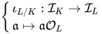
授業の延長 を代数体( 基底体 と呼ばれる)とし 、を 有限次数の体拡大とする。 と をそれぞれ 整数環、非零分数イデアル群、体の主分数イデアルの部分群とする 。すると、分数イデアルの拡大写像は
け
{\displaystyle K}
ら
/
け
{\displaystyle L/K}
お
け
、
私
け
、
ポ
け
{\displaystyle {\mathcal {O}}_{K},{\mathcal {I}}_{K},{\mathcal {P}}_{K}}
お
ら
、
私
ら
、
ポ
ら
{\displaystyle {\mathcal {O}}_{L}、{\mathcal {I}}_{L}、{\mathcal {P}}_{L}}
け 、 ら
{\displaystyle K,L}
{
ι
ら
/
け
:
私
け
→
私
ら
1つの
↦
1つの
お
ら
{\displaystyle {\begin{cases}\iota _{L/K}:{\mathcal {I}}_{K}\to {\mathcal {I}}_{L}\\{\mathfrak {a}}\mapsto {\mathfrak {a}}{\mathcal {O}}_{L}\end{cases}}}
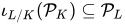
は、入射的な 群準同型 である。 なので 、この写像は イデアル類群 の拡大準同型を誘導する。
ι
ら
/
け
(
ポ
け
) ⊆
ポ
ら
{\displaystyle \iota _{L/K}({\mathcal {P}}_{K})\subseteq {\mathcal {P}}_{L}}
{
じゅう
ら
/
け
:
私
け
/
ポ
け
→
私
ら
/
ポ
ら
1つの
ポ
け
↦ (
1つの
お
ら
)
ポ
ら
{\displaystyle {\begin{cases}j_{L/K}:{\mathcal {I}}_{K}/{\mathcal {P}}_{K}\to {\mathcal {I}}_{L}/{\mathcal {P}}_{L}\\{\mathfrak {a}}{\mathcal {P}}_{K}\mapsto ({\mathfrak {a}}{\mathcal {O}}_{L}){\mathcal {P}}_{L}\end{cases}}}
非主イデアル (つまり ) が存在し、その拡大イデアルが 主 (つまり、 ある およびに対して ) である場合、 における プリンシパル化 または 降伏 について語ります。この場合、イデアル とそのクラスは において プリンシパル化 または 降伏する と言われます。この現象は、 クラス拡大準同型の
核 である プリンシパル化核 または 降伏核 によって最も便利に記述されます。
1つの
∈
私
け
{\displaystyle {\mathfrak {a}}\in {\mathcal {I}}_{K}}
1つの
ポ
け
≠
ポ
け
{\displaystyle {\mathfrak {a}}{\mathcal {P}}_{K}\neq {\mathcal {P}}_{K}}
ら
{\displaystyle L}
1つの
お
ら
= あ
お
ら
{\displaystyle {\mathfrak {a}}{\mathcal {O}}_{L}=A{\mathcal {O}}_{L}}
あ ∈
お
ら
{\displaystyle A\in {\mathcal {O}}_{L}}
(
a
O
L
)
P
L
=
(
A
O
L
)
P
L
=
P
L
{\displaystyle ({\mathfrak {a}}{\mathcal {O}}_{L}){\mathcal {P}}_{L}=(A{\mathcal {O}}_{L}){\mathcal {P}}_{L}={\mathcal {P}}_{L}}
L
/
K
{\displaystyle L/K}
a
{\displaystyle {\mathfrak {a}}}
a
P
K
{\displaystyle {\mathfrak {a}}{\mathcal {P}}_{K}}
L
{\displaystyle L}
ker
(
j
L
/
K
)
{\displaystyle \ker(j_{L/K})}
より一般的には、を の 法とし 、 は の 非ゼロイデアル であり 、 は の異なる 実無限素数 の形式積で あるとする 。すると、
m
=
m
0
m
∞
{\displaystyle {\mathfrak {m}}={\mathfrak {m}}_{0}{\mathfrak {m}}_{\infty }}
K
{\displaystyle K}
m
0
{\displaystyle {\mathfrak {m}}_{0}}
O
K
{\displaystyle {\mathcal {O}}_{K}}
m
∞
{\displaystyle {\mathfrak {m}}_{\infty }}
K
{\displaystyle K}
S
K
,
m
=
⟨
α
O
K
|
α
≡
1
mod
m
⟩
≤
I
K
(
m
)
,
{\displaystyle {\mathcal {S}}_{K,{\mathfrak {m}}}=\langle \alpha {\mathcal {O}}_{K}|\alpha \equiv 1{\bmod {\mathfrak {m}}}\rangle \leq {\mathcal {I}}_{K}({\mathfrak {m}}),}
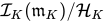
はを 法とする 射線 で 、 はと 互いに素な における 非ゼロ分数イデアルの群であり 、条件は を割り切る すべての実無限素数 に対して および を 意味する。 すると、群は に対する 一般化イデアル類群と 呼ばれる。および が、 任意の に対して で あり、 任意の に対して となる一般化イデアル類群である 場合 、 は 一般化イデアル類群の拡張準同型性を誘導する。
m
{\displaystyle {\mathfrak {m}}}
I
K
(
m
)
=
I
K
(
m
0
)
{\displaystyle {\mathcal {I}}_{K}({\mathfrak {m}})={\mathcal {I}}_{K}({\mathfrak {m}}_{0})}
K
{\displaystyle K}
m
0
{\displaystyle {\mathfrak {m}}_{0}}
α
≡
1
mod
m
{\displaystyle \alpha \equiv 1{\bmod {\mathfrak {m}}}}
α
≡
1
mod
m
0
{\displaystyle \alpha \equiv 1{\bmod {{\mathfrak {m}}_{0}}}}
v
(
α
)
>
0
{\displaystyle v(\alpha )>0}
v
{\displaystyle v}
m
∞
.
{\displaystyle {\mathfrak {m}}_{\infty }.}
S
K
,
m
≤
H
≤
I
K
(
m
)
,
{\displaystyle {\mathcal {S}}_{K,{\mathfrak {m}}}\leq {\mathcal {H}}\leq {\mathcal {I}}_{K}({\mathfrak {m}}),}
I
K
(
m
)
/
H
{\displaystyle {\mathcal {I}}_{K}({\mathfrak {m}})/{\mathcal {H}}}
m
.
{\displaystyle {\mathfrak {m}}.}
I
K
(
m
K
)
/
H
K
{\displaystyle {\mathcal {I}}_{K}({\mathfrak {m}}_{K})/{\mathcal {H}}_{K}}
I
L
(
m
L
)
/
H
L
{\displaystyle {\mathcal {I}}_{L}({\mathfrak {m}}_{L})/{\mathcal {H}}_{L}}
a
O
L
∈
I
L
(
m
L
)
{\displaystyle {\mathfrak {a}}{\mathcal {O}}_{L}\in {\mathcal {I}}_{L}({\mathfrak {m}}_{L})}
a
∈
I
K
(
m
K
)
{\displaystyle {\mathfrak {a}}\in {\mathcal {I}}_{K}({\mathfrak {m}}_{K})}
a
O
L
∈
H
L
{\displaystyle {\mathfrak {a}}{\mathcal {O}}_{L}\in {\mathcal {H}}_{L}}
a
∈
H
K
{\displaystyle {\mathfrak {a}}\in {\mathcal {H}}_{K}}
ι
L
/
K
{\displaystyle \iota _{L/K}}
{
j
L
/
K
:
I
K
(
m
K
)
/
H
K
→
I
L
(
m
L
)
/
H
L
a
H
K
↦
(
a
O
L
)
H
L
{\displaystyle {\begin{cases}j_{L/K}:{\mathcal {I}}_{K}({\mathfrak {m}}_{K})/{\mathcal {H}}_{K}\to {\mathcal {I}}_{L}({\mathfrak {m}}_{L})/{\mathcal {H}}_{L}\\{\mathfrak {a}}{\mathcal {H}}_{K}\mapsto ({\mathfrak {a}}{\mathcal {O}}_{L}){\mathcal {H}}_{L}\end{cases}}}
数体のガロア拡大 をガロア群 を持つ代数体の ガロア拡大 とし 、 をそれぞれ の体の素イデアルの集合を表すものとします 。 は の 素イデアル で あり、 相対判別式 を割り切れないため において 不分岐 で あるとし 、 は 上にある の素イデアルとします 。
F
/
K
{\displaystyle F/K}
G
=
G
a
l
(
F
/
K
)
{\displaystyle G=\mathrm {Gal} (F/K)}
P
K
,
P
F
{\displaystyle \mathbb {P} _{K},\mathbb {P} _{F}}
K
,
F
{\displaystyle K,F}
p
∈
P
K
{\displaystyle {\mathfrak {p}}\in \mathbb {P} _{K}}
K
{\displaystyle K}
d
=
d
(
F
/
K
)
{\displaystyle {\mathfrak {d}}={\mathfrak {d}}(F/K)}
F
{\displaystyle F}
P
∈
P
F
{\displaystyle {\mathfrak {P}}\in \mathbb {P} _{F}}
F
{\displaystyle F}
p
{\displaystyle {\mathfrak {p}}}
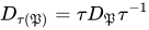
フロベニウス自己同型 すべての代数的整数 に対して 、 となる 一意の自己同型が存在する。ここで は の ノルム である。この写像は の フロベニウス自己同型 と呼ばれる 。これは の 分解群を 生成し、その位数は上の の 慣性次数 に等しい 。( が分岐している場合、 は 定義され、 慣性部分群 を法としてを生成する。
σ
∈
G
{\displaystyle \sigma \in G}
A
N
(
p
)
≡
σ
(
A
)
mod
P
{\displaystyle A^{\mathrm {N} ({\mathfrak {p}})}\equiv \sigma (A){\bmod {\mathfrak {P}}}}
A
∈
O
F
{\displaystyle A\in {\mathcal {O}}_{F}}
N
(
p
)
{\displaystyle \mathrm {N} ({\mathfrak {p}})}
p
{\displaystyle {\mathfrak {p}}}
[
F
/
K
P
]
:=
σ
{\textstyle \left[{\frac {F/K}{\mathfrak {P}}}\right]:=\sigma }
P
{\displaystyle {\mathfrak {P}}}
D
P
=
{
σ
∈
G
|
σ
(
P
)
=
P
}
{\displaystyle D_{\mathfrak {P}}=\{\sigma \in G|\sigma ({\mathfrak {P}})={\mathfrak {P}}\}}
P
{\displaystyle {\mathfrak {P}}}
f
:=
f
(
P
|
p
)
=
[
O
F
/
P
:
O
K
/
p
]
{\displaystyle f:=f({\mathfrak {P}}|{\mathfrak {p}})=[{\mathcal {O}}_{F}/{\mathfrak {P}}:{\mathcal {O}}_{K}/{\mathfrak {p}}]}
P
{\displaystyle {\mathfrak {P}}}
p
{\displaystyle {\mathfrak {p}}}
p
{\displaystyle {\mathfrak {p}}}
[
F
/
K
P
]
{\textstyle \left[{\frac {F/K}{\mathfrak {P}}}\right]}
D
P
{\displaystyle D_{\mathfrak {P}}}
I
P
=
{
σ
∈
G
|
σ
(
A
)
≡
A
mod
P
for all
A
∈
O
F
}
=
ker
(
D
P
→
G
a
l
(
O
F
/
P
|
O
K
/
p
)
)
{\displaystyle I_{\mathfrak {P}}=\{\sigma \in G|\sigma (A)\equiv A{\bmod {\mathfrak {P}}}{\text{ for all }}A\in {\mathcal {O}}_{F}\}=\ker(D_{\mathfrak {P}}\to \mathrm {Gal} ({\mathcal {O}}_{F}/{\mathfrak {P}}|{\mathcal {O}}_{K}/{\mathfrak {p}}))}
の位数は 上 の の 分岐指数 である。 を割り切るの他の任意の素イデアルは のある の 形をとる 。そのフロベニウス自己同型は次のように与えられる。
e
(
P
|
p
)
{\displaystyle e({\mathfrak {P}}|{\mathfrak {p}})}
P
{\displaystyle {\mathfrak {P}}}
p
{\displaystyle {\mathfrak {p}}}
F
{\displaystyle F}
p
{\displaystyle {\mathfrak {p}}}
τ
(
P
)
{\displaystyle \tau ({\mathfrak {P}})}
τ
∈
G
{\displaystyle \tau \in G}
[
F
/
K
τ
(
P
)
]
=
τ
[
F
/
K
P
]
τ
−
1
,
{\displaystyle \left[{\frac {F/K}{\tau ({\mathfrak {P}})}}\right]=\tau \left[{\frac {F/K}{\mathfrak {P}}}\right]\tau ^{-1},}
以来
τ
(
A
)
N
(
p
)
≡
(
τ
σ
τ
−
1
)
(
τ
(
A
)
)
mod
τ
(
P
)
{\displaystyle \tau (A)^{\mathrm {N} ({\mathfrak {p}})}\equiv (\tau \sigma \tau ^{-1})(\tau (A)){\bmod {\tau ({\mathfrak {P}})}}}
であり 、したがってその分解群は と共役である 。この一般的な状況では、 アルティン記号 は写像である。
A
∈
O
F
{\displaystyle A\in {\mathcal {O}}_{F}}
D
τ
(
P
)
=
τ
D
P
τ
−
1
{\displaystyle D_{\tau ({\mathfrak {P}})}=\tau D_{\mathfrak {P}}\tau ^{-1}}
D
P
{\displaystyle D_{\mathfrak {P}}}
p
↦
(
F
/
K
p
)
:=
{
τ
[
F
/
K
P
]
τ
−
1
|
τ
∈
G
}
{\displaystyle {\mathfrak {p}}\mapsto \left({\frac {F/K}{\mathfrak {p}}}\right):=\left.\left\{\tau \left[{\frac {F/K}{\mathfrak {P}}}\right]\tau ^{-1}\right|\tau \in G\right\}}
これは、自己同型の共役類 全体 を任意の非分岐素イデアルに関連付け 、 が 完全に で分解される 場合に限り、が成り立ちます 。
p
∤
d
{\displaystyle {\mathfrak {p}}\nmid {\mathfrak {d}}}
(
F
/
K
p
)
=
1
{\textstyle \left({\frac {F/K}{\mathfrak {p}}}\right)=1}
p
{\displaystyle {\mathfrak {p}}}
F
{\displaystyle F}
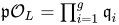
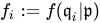
素イデアルの因数分解 が相対ガロア群 を持つ中間体である 場合 、 (ただしは上記のように で不分岐 )の での因数分解を 次のように での因数分解から 構成できるため 、準同型および についてのより正確な記述が可能になります。 [1] [2] 上 の素イデアルは、 左剰余類の -集合 と 同変 単射であり 、 は 剰余類 に対応します 。 上の すべての素イデアルに対して、 ガロア群は 上の 素イデアルの集合に推移的に作用するため 、このようなイデアルは、 の左乗法による へ の作用の軌道と単射です。このような軌道は、さらに、 二重剰余類 と単射です 。 をこれらの二重剰余類の代表の完全なシステムとすると、 になります 。さらに、の 左剰余類の集合へ の作用における 剰余類の軌道を で左乗法で表し、の 右剰余類の集合へ の作用における 剰余類の軌道を で右乗法で表します。次に 、 を として 因数分解します。ここで、の 素イデアルは の任意の代表システム上で実行される積 を 満たし、 の上にある素イデアルです 。
K
⊆
L
⊆
F
{\displaystyle K\subseteq L\subseteq F}
H
=
G
a
l
(
F
/
L
)
≤
G
{\displaystyle H=\mathrm {Gal} (F/L)\leq G}
ι
L
/
K
{\displaystyle \iota _{L/K}}
j
L
/
K
{\displaystyle j_{L/K}}
p
{\displaystyle {\mathfrak {p}}}
p
{\displaystyle {\mathfrak {p}}}
F
{\displaystyle F}
O
L
{\displaystyle {\mathcal {O}}_{L}}
O
F
{\displaystyle {\mathcal {O}}_{F}}
O
F
{\displaystyle {\mathcal {O}}_{F}}
p
{\displaystyle {\mathfrak {p}}}
G
{\displaystyle G}
G
{\displaystyle G}
G
/
D
P
{\displaystyle G/D_{\mathfrak {P}}}
τ
(
P
)
{\displaystyle \tau ({\mathfrak {P}})}
τ
D
P
{\displaystyle \tau D_{\mathfrak {P}}}
q
{\displaystyle {\mathfrak {q}}}
O
L
{\displaystyle {\mathcal {O}}_{L}}
p
{\displaystyle {\mathfrak {p}}}
H
{\displaystyle H}
O
F
{\displaystyle {\mathcal {O}}_{F}}
q
{\displaystyle {\mathfrak {q}}}
q
{\displaystyle {\mathfrak {q}}}
H
{\displaystyle H}
G
/
D
P
{\displaystyle G/D_{\mathfrak {P}}}
H
∖
G
/
D
P
{\displaystyle H\backslash G/D_{\mathfrak {P}}}
(
τ
1
,
…
,
τ
g
)
{\displaystyle (\tau _{1},\ldots ,\tau _{g})}
G
=
∪
˙
i
=
1
g
H
τ
i
D
P
{\displaystyle G={\dot {\cup }}_{i=1}^{g}\,H\tau _{i}D_{\mathfrak {P}}}
H
⋅
τ
i
D
P
{\displaystyle H\cdot \tau _{i}D_{\mathfrak {P}}}
τ
i
D
P
{\displaystyle \tau _{i}D_{\mathfrak {P}}}
H
{\displaystyle H}
G
/
D
P
{\displaystyle G/D_{\mathfrak {P}}}
H
τ
i
⋅
D
P
{\displaystyle H\tau _{i}\cdot D_{\mathfrak {P}}}
H
τ
i
{\displaystyle H\tau _{i}}
D
P
{\displaystyle D_{\mathfrak {P}}}
H
∖
G
{\displaystyle H\backslash G}
p
{\displaystyle {\mathfrak {p}}}
O
L
{\displaystyle {\mathcal {O}}_{L}}
p
O
L
=
∏
i
=
1
g
q
i
{\textstyle {\mathfrak {p}}{\mathcal {O}}_{L}=\prod _{i=1}^{g}{\mathfrak {q}}_{i}}
q
i
∈
P
L
{\displaystyle {\mathfrak {q}}_{i}\in \mathbb {P} _{L}}
1
≤
i
≤
g
{\displaystyle 1\leq i\leq g}
p
{\displaystyle {\mathfrak {p}}}
L
{\displaystyle L}
q
i
O
F
=
∏
ϱ
ϱ
(
P
)
{\textstyle {\mathfrak {q}}_{i}{\mathcal {O}}_{F}=\prod _{\varrho }\varrho ({\mathfrak {P}})}
H
⋅
τ
i
D
P
{\displaystyle H\cdot \tau _{i}D_{\mathfrak {P}}}
我々は持っています
#
(
H
⋅
τ
i
D
P
)
⋅
#
D
P
=
#
H
τ
i
D
P
=
#
(
H
τ
i
⋅
D
P
)
⋅
#
H
.
{\displaystyle \#(H\cdot \tau _{i}D_{\mathfrak {P}})\cdot \#D_{\mathfrak {P}}=\#H\tau _{i}D_{\mathfrak {P}}=\#(H\tau _{i}\cdot D_{\mathfrak {P}})\cdot \#H.}
を 上 の の分解群と します 。すると は の 上 の作用における の安定群なので、 軌道安定定理 によりが 成り立ちます 。一方 は であり、 これらを合わせると
D
i
{\displaystyle D_{i}}
τ
i
(
P
)
{\displaystyle \tau _{i}({\mathfrak {P}})}
L
{\displaystyle L}
D
i
=
H
∩
D
τ
i
(
P
)
{\displaystyle D_{i}=H\cap D_{\tau _{i}({\mathfrak {P}})}}
τ
i
D
P
{\displaystyle \tau _{i}D_{\mathfrak {P}}}
H
{\displaystyle H}
G
/
D
P
{\displaystyle G/D_{\mathfrak {P}}}
#
D
i
=
#
H
/
#
(
H
⋅
τ
i
D
P
)
{\displaystyle \#D_{i}=\#H/\#(H\cdot \tau _{i}D_{\mathfrak {P}})}
#
D
i
=
f
(
τ
i
(
P
)
|
q
i
)
{\displaystyle \#D_{i}=f(\tau _{i}({\mathfrak {P}})|{\mathfrak {q}}_{i})}
f
(
q
i
|
p
)
=
f
(
τ
i
(
P
)
|
p
)
f
(
τ
i
(
P
)
|
q
i
)
=
f
(
P
|
p
)
#
D
i
=
#
D
P
#
H
/
#
(
H
⋅
τ
i
D
P
)
=
#
(
H
⋅
τ
i
D
P
)
⋅
#
D
P
#
H
=
#
H
τ
i
D
P
#
H
=
#
(
H
τ
i
⋅
D
P
)
.
{\displaystyle f({\mathfrak {q}}_{i}|{\mathfrak {p}})={\frac {f(\tau _{i}({\mathfrak {P}})|{\mathfrak {p}})}{f(\tau _{i}({\mathfrak {P}})|{\mathfrak {q}}_{i})}}={\frac {f({\mathfrak {P}}|{\mathfrak {p}})}{\#D_{i}}}={\frac {\#D_{\mathfrak {P}}}{\#H/\#(H\cdot \tau _{i}D_{\mathfrak {P}})}}={\frac {\#(H\cdot \tau _{i}D_{\mathfrak {P}})\cdot \#D_{\mathfrak {P}}}{\#H}}={\frac {\#H\tau _{i}D_{\mathfrak {P}}}{\#H}}=\#(H\tau _{i}\cdot D_{\mathfrak {P}}).}
言い換えれば、慣性次数は、右乗法による 右剰余類の集合へ の の作用における 剰余類の軌道のサイズに等しい。逆をとると、これは、左乗法による 左剰余類の集合への の作用における 剰余類の 軌道のサイズに等しい。また、 の上 の素イデアルは この作用の軌道に対応している。
f
i
:=
f
(
q
i
|
p
)
{\displaystyle f_{i}:=f({\mathfrak {q}}_{i}|{\mathfrak {p}})}
H
τ
i
{\displaystyle H\tau _{i}}
[
F
/
K
P
]
{\textstyle \left[{\frac {F/K}{\mathfrak {P}}}\right]}
H
∖
G
{\displaystyle H\backslash G}
D
P
⋅
τ
i
−
1
H
{\displaystyle D_{\mathfrak {P}}\cdot \tau _{i}^{-1}H}
τ
i
−
1
H
{\displaystyle \tau _{i}^{-1}H}
[
F
/
K
P
]
{\textstyle \left[{\frac {F/K}{\mathfrak {P}}}\right]}
G
/
H
{\displaystyle G/H}
O
L
{\displaystyle {\mathcal {O}}_{L}}
p
{\displaystyle {\mathfrak {p}}}
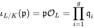
その結果、理想的な埋め込みは で与えられ 、クラス拡張は で与えられる。
ι
L
/
K
(
p
)
=
p
O
L
=
∏
i
=
1
g
q
i
{\textstyle \iota _{L/K}({\mathfrak {p}})={\mathfrak {p}}{\mathcal {O}}_{L}=\prod _{i=1}^{g}{\mathfrak {q}}_{i}}
j
L
/
K
(
p
H
K
)
=
(
p
O
L
)
H
L
=
∏
i
=
1
g
q
i
H
L
.
{\displaystyle j_{L/K}({\mathfrak {p}}{\mathcal {H}}_{K})=({\mathfrak {p}}{\mathcal {O}}_{L}){\mathcal {H}}_{L}=\prod _{i=1}^{g}{\mathfrak {q}}_{i}{\mathcal {H}}_{L}.}
アルティンの相互法則 ここでさらに、 が アーベル拡大 、つまり が アーベル群であると仮定します。すると、 上 にある の素イデアルのすべての共役分解群は一致するため 、 任意の に対してとなり 、アルティン記号は 任意の のフロベニウス自己同型に等しくなり、 すべての および任意の に対して と なり ます 。
F
/
K
{\displaystyle F/K}
G
{\displaystyle G}
F
{\displaystyle F}
p
{\displaystyle {\mathfrak {p}}}
D
p
:=
D
τ
(
P
)
{\displaystyle D_{\mathfrak {p}}:=D_{\tau ({\mathfrak {P}})}}
τ
∈
G
{\displaystyle \tau \in G}
(
F
/
K
p
)
=
[
F
/
K
P
]
{\textstyle \left({\frac {F/K}{\mathfrak {p}}}\right)=\left[{\frac {F/K}{\mathfrak {P}}}\right]}
P
∣
p
{\displaystyle {\mathfrak {P}}\mid {\mathfrak {p}}}
A
N
(
p
)
≡
(
F
/
K
p
)
(
A
)
mod
P
{\textstyle A^{\mathrm {N} ({\mathfrak {p}})}\equiv \left({\frac {F/K}{\mathfrak {p}}}\right)(A){\bmod {\mathfrak {P}}}}
A
∈
O
F
{\displaystyle A\in {\mathcal {O}}_{F}}
P
∣
p
{\displaystyle {\mathfrak {P}}\mid {\mathfrak {p}}}
類体理論 [3] によれば 、
アーベル拡大は と を法とする 射線 の間の 中間群に一意に対応する 。ここで は 相対 導体を 表す( は と同じ素イデアルで割り切れる )。アルティン記号
F
/
K
{\displaystyle F/K}
S
K
,
f
≤
H
≤
I
K
(
f
)
{\displaystyle {\mathcal {S}}_{K,{\mathfrak {f}}}\leq {\mathcal {H}}\leq {\mathcal {I}}_{K}({\mathfrak {f}})}
f
{\displaystyle {\mathfrak {f}}}
K
{\displaystyle K}
I
K
(
f
)
{\displaystyle {\mathcal {I}}_{K}({\mathfrak {f}})}
f
=
f
0
f
∞
=
f
(
F
/
K
)
{\displaystyle {\mathfrak {f}}={\mathfrak {f}}_{0}{\mathfrak {f}}_{\infty }={\mathfrak {f}}(F/K)}
f
0
{\displaystyle {\mathfrak {f}}_{0}}
d
{\displaystyle {\mathfrak {d}}}
{
P
K
(
f
)
→
G
p
↦
(
F
/
K
p
)
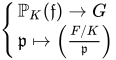
{\displaystyle {\begin{cases}\mathbb {P} _{K}({\mathfrak {f}})\to G\\{\mathfrak {p}}\mapsto \left({\frac {F/K}{\mathfrak {p}}}\right)\end{cases}}}
のフロベニウス自己同型を の 非分岐な 各素イデアルに関連付ける 。これは乗法的に全射準同型に拡張できる。
p
{\displaystyle {\mathfrak {p}}}
p
{\displaystyle {\mathfrak {p}}}
K
{\displaystyle K}
F
{\displaystyle F}
{
I
K
(
f
)
→
G
a
=
∏
p
v
p
(
a
)
↦
(
F
/
K
a
)
:=
∏
(
F
/
K
p
)
v
p
(
a
)
{\displaystyle {\begin{cases}{\mathcal {I}}_{K}({\mathfrak {f}})\to G\\{\mathfrak {a}}=\prod {\mathfrak {p}}^{v_{\mathfrak {p}}({\mathfrak {a}})}\mapsto \left({\frac {F/K}{\mathfrak {a}}}\right):=\prod \left({\frac {F/K}{\mathfrak {p}}}\right)^{v_{\mathfrak {p}}({\mathfrak {a}})}\end{cases}}}
核 (ここで は を意味する )は アルティン写像 と呼ばれ、同型写像を誘導する。
H
=
S
K
,
f
⋅
N
F
/
K
(
I
F
(
f
)
)
{\displaystyle {\mathcal {H}}={\mathcal {S}}_{K,{\mathfrak {f}}}\cdot \mathrm {N} _{F/K}({\mathcal {I}}_{F}({\mathfrak {f}}))}
I
F
(
f
)
{\displaystyle {\mathcal {I}}_{F}({\mathfrak {f}})}
I
F
(
f
0
O
F
)
{\displaystyle {\mathcal {I}}_{F}({\mathfrak {f}}_{0}{\mathcal {O}}_{F})}
{
I
K
(
f
)
/
H
→
G
=
G
a
l
(
F
/
K
)
a
H
↦
(
F
/
K
a
)
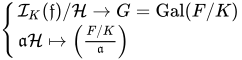
{\displaystyle {\begin{cases}{\mathcal {I}}_{K}({\mathfrak {f}})/{\mathcal {H}}\to G=\mathrm {Gal} (F/K)\\{\mathfrak {a}}{\mathcal {H}}\mapsto \left({\frac {F/K}{\mathfrak {a}}}\right)\end{cases}}}
一般化イデアル類群の ガロア群への同型性。この明示的な同型性は アルティンの相互法則 または 一般相互法則 と呼ばれる 。 [4]
I
K
(
f
)
/
H
{\displaystyle {\mathcal {I}}_{K}({\mathfrak {f}})/{\mathcal {H}}}
G
{\displaystyle G}
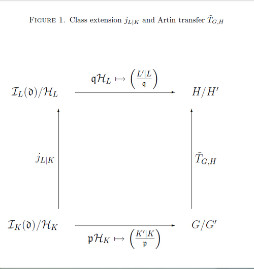
図 1: クラス拡張とアルティン転送を結び付ける可換図。
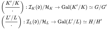
この相互法則により、アルティンは、次のシナリオに基づいて、 数体に対する 一般主化問題を 数論から群論に翻訳することができました。 を 自己同型群 を持つ代数的数体のガロア拡大とします 。 を 相対群 を持つ中間体と仮定し 、 を の範囲内で の の最大アーベル部分拡大とします 。すると、対応する相対群はそれぞれ 交換子部分群 、です。類体理論により、 アルティン写像が同型を確立する
中間群 および が存在し、
K
⊆
L
⊆
F
{\displaystyle K\subseteq L\subseteq F}
F
/
K
{\displaystyle F/K}
G
=
G
a
l
(
F
/
K
)
{\displaystyle G=\mathrm {Gal} (F/K)}
K
⊆
L
⊆
F
{\displaystyle K\subseteq L\subseteq F}
H
=
G
a
l
(
F
/
L
)
≤
G
{\displaystyle H=\mathrm {Gal} (F/L)\leq G}
K
′
/
K
,
L
′
/
L
{\displaystyle K'/K,L'/L}
K
,
L
{\displaystyle K,L}
F
{\displaystyle F}
G
′
=
G
a
l
(
F
/
K
′
)
≤
G
{\displaystyle G'=\mathrm {Gal} (F/K')\leq G}
H
′
=
G
a
l
(
F
/
L
′
)
≤
H
{\displaystyle H'=\mathrm {Gal} (F/L')\leq H}
S
K
,
m
K
≤
H
K
≤
I
K
(
d
)
{\displaystyle {\mathcal {S}}_{K,{\mathfrak {m}}_{K}}\leq {\mathcal {H}}_{K}\leq {\mathcal {I}}_{K}({\mathfrak {d}})}
S
L
,
m
L
≤
H
L
≤
I
L
(
d
)
{\displaystyle {\mathcal {S}}_{L,{\mathfrak {m}}_{L}}\leq {\mathcal {H}}_{L}\leq {\mathcal {I}}_{L}({\mathfrak {d}})}
(
K
′
/
K
⋅
)
:
I
K
(
d
)
/
H
K
→
G
a
l
(
K
′
/
K
)
≃
G
/
G
′
(
L
′
/
L
⋅
)
:
I
L
(
d
)
/
H
L
→
G
a
l
(
L
′
/
L
)
≃
H
/
H
′
{\displaystyle {\begin{aligned}&\left({\frac {K'/K}{\cdot }}\right):{\mathcal {I}}_{K}({\mathfrak {d}})/{\mathcal {H}}_{K}\to \mathrm {Gal} (K'/K)\simeq G/G'\\&\left({\frac {L'/L}{\cdot }}\right):{\mathcal {I}}_{L}({\mathfrak {d}})/{\mathcal {H}}_{L}\to \mathrm {Gal} (L'/L)\simeq H/H'\end{aligned}}}
ここで、 は それぞれ で割り切れる法、 はそれぞれ を割り切るすべての素数で 割り切れる法であること を意味します 。
d
=
d
(
F
/
K
)
,
I
L
(
d
)
{\displaystyle {\mathfrak {d}}={\mathfrak {d}}(F/K),{\mathcal {I}}_{L}({\mathfrak {d}})}
I
L
(
d
O
L
)
{\displaystyle {\mathcal {I}}_{L}({\mathfrak {d}}{\mathcal {O}}_{L})}
m
K
,
m
L
{\displaystyle {\mathfrak {m}}_{K},{\mathfrak {m}}_{L}}
f
(
K
′
/
K
)
,
f
(
L
′
/
L
)
{\displaystyle {\mathfrak {f}}(K'/K),{\mathfrak {f}}(L'/L)}
d
,
d
O
L
{\displaystyle {\mathfrak {d}},{\mathfrak {d}}{\mathcal {O}}_{L}}
理想的な拡大準同型 、 誘導アルティン転移 、およびこれらのアルティン写像は、次の式で結びついている。
ι
L
/
K
:
I
K
(
d
)
→
I
L
(
d
)
{\displaystyle \iota _{L/K}:\,{\mathcal {I}}_{K}({\mathfrak {d}})\to {\mathcal {I}}_{L}({\mathfrak {d}})}
T
~
G
,
H
{\displaystyle {\tilde {T}}_{G,H}}
T
~
G
,
H
∘
(
K
′
/
K
⋅
)
=
(
L
′
/
L
⋅
)
∘
ι
L
/
K
.
{\displaystyle {\tilde {T}}_{G,H}\circ \left({\frac {K'/K}{\cdot }}\right)=\left({\frac {L'/L}{\cdot }}\right)\circ \iota _{L/K}.}
はを割り切れない の素イデアルによって生成される ので 、これらの生成元でこの等式を検証すれば十分です。したがって、 が を割り切れない の素イデアルであるとし 、が 上にある の素イデアルであるとします 。一方で、イデアル拡大準同型は 、基本体の イデアルを 体 の 拡大イデアルに写し、 体の アルティン写像は 、この素イデアルの積をフロベニウス自己同型の共役の積に写します。
I
K
(
d
)
{\displaystyle {\mathcal {I}}_{K}({\mathfrak {d}})}
K
{\displaystyle K}
d
{\displaystyle {\mathfrak {d}}}
p
∈
P
K
{\displaystyle {\mathfrak {p}}\in \mathbb {P} _{K}}
K
{\displaystyle K}
d
{\displaystyle {\mathfrak {d}}}
P
∈
P
F
{\displaystyle {\mathfrak {P}}\in \mathbb {P} _{F}}
F
{\displaystyle F}
p
{\displaystyle {\mathfrak {p}}}
ι
L
/
K
{\displaystyle \iota _{L/K}}
p
{\displaystyle {\mathfrak {p}}}
K
{\displaystyle K}
ι
L
/
K
(
p
)
=
p
O
L
=
∏
i
=
1
g
q
i
{\displaystyle \iota _{L/K}({\mathfrak {p}})={\mathfrak {p}}{\mathcal {O}}_{L}=\prod _{i=1}^{g}{\mathfrak {q}}_{i}}
L
{\displaystyle L}
(
L
′
/
L
⋅
)
{\textstyle \left({\frac {L'/L}{\cdot }}\right)}
L
{\displaystyle L}
∏
i
=
1
g
(
L
′
/
L
q
i
)
=
∏
i
=
1
g
[
F
/
L
τ
i
(
P
)
]
⋅
H
′
=
∏
i
=
1
g
τ
i
[
F
/
L
P
]
τ
i
−
1
⋅
H
′
=
∏
i
=
1
g
τ
i
[
F
/
K
P
]
f
i
τ
i
−
1
⋅
H
′
,
{\displaystyle \prod _{i=1}^{g}\left({\frac {L'/L}{{\mathfrak {q}}_{i}}}\right)=\prod _{i=1}^{g}\left[{\frac {F/L}{\tau _{i}({\mathfrak {P}})}}\right]\cdot H'=\prod _{i=1}^{g}\tau _{i}\left[{\frac {F/L}{\mathfrak {P}}}\right]\tau _{i}^{-1}\cdot H'=\prod _{i=1}^{g}\tau _{i}\left[{\frac {F/K}{\mathfrak {P}}}\right]^{f_{i}}\tau _{i}^{-1}\cdot H',}
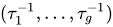
ここで、ここで使用される二重剰余類分解とその代表は、前々節で使用したのと同じである。一方、 基底体のアルティン写像は 、イデアルを フロベニウス自己同型に写像する 。 -組は、 二重剰余類の代表のシステムであり、左乗法による 左剰余類の集合へ の作用の軌道に対応し 、この作用における 剰余類の軌道のサイズに等しい 。したがって、誘導アルティン転送は、積に写像される 。
(
K
′
/
K
⋅
)
{\textstyle \left({\frac {K'/K}{\cdot }}\right)}
K
{\displaystyle K}
p
{\displaystyle {\mathfrak {p}}}
(
K
′
/
K
p
)
=
[
F
/
K
P
]
⋅
G
′
{\textstyle \left({\frac {K'/K}{\mathfrak {p}}}\right)=\left[{\frac {F/K}{\mathfrak {P}}}\right]\cdot G'}
g
{\displaystyle g}
(
τ
1
−
1
,
…
,
τ
g
−
1
)
{\displaystyle (\tau _{1}^{-1},\ldots ,\tau _{g}^{-1})}
D
P
∖
G
/
H
{\displaystyle D_{\mathfrak {P}}\backslash G/H}
[
F
/
K
P
]
{\textstyle \left[{\frac {F/K}{\mathfrak {P}}}\right]}
G
/
H
{\displaystyle G/H}
f
i
=
#
(
H
τ
i
⋅
D
P
)
=
#
(
D
P
⋅
τ
i
−
1
H
)
{\displaystyle f_{i}=\#(H\tau _{i}\cdot D_{\mathfrak {P}})=\#(D_{\mathfrak {P}}\cdot \tau _{i}^{-1}H)}
τ
i
−
1
H
{\displaystyle \tau _{i}^{-1}H}
[
F
/
K
P
]
⋅
G
′
{\textstyle \left[{\frac {F/K}{\mathfrak {P}}}\right]\cdot G'}
T
~
G
,
H
(
[
F
/
K
P
]
⋅
G
′
)
=
T
G
,
H
(
[
F
/
K
P
]
)
=
∏
i
=
1
g
(
τ
i
−
1
)
−
1
[
F
/
K
P
]
f
i
τ
i
−
1
⋅
H
′
=
∏
i
=
1
g
τ
i
[
F
/
K
P
]
f
i
τ
i
−
1
⋅
H
′
.
{\displaystyle {\tilde {T}}_{G,H}\left(\left[{\frac {F/K}{\mathfrak {P}}}\right]\cdot G'\right)=T_{G,H}\left(\left[{\frac {F/K}{\mathfrak {P}}}\right]\right)=\prod _{i=1}^{g}(\tau _{i}^{-1})^{-1}\left[{\frac {F/K}{\mathfrak {P}}}\right]^{f_{i}}\tau _{i}^{-1}\cdot H'=\prod _{i=1}^{g}\tau _{i}\left[{\frac {F/K}{\mathfrak {P}}}\right]^{f_{i}}\tau _{i}^{-1}\cdot H'.}
この積表現はアルティン転送準同型の元の形であり、 置換表現を 互いに素なサイクル に分解したものに相当する 。 [5]
アルティン写像と の核はそれぞれ と なので 、前の式は を意味します 。したがって、類拡張準同型が存在し 、 と誘導アルティン転送は、 アルティン写像によって誘導される同型を介して図 1 の可換図で接続されます。つまり、2 つの合成 の等式が成り立ちます 。 [3] [6]
(
K
′
/
K
⋅
)
{\displaystyle \left({\tfrac {K'/K}{\cdot }}\right)}
(
L
′
/
L
⋅
)
{\displaystyle \left({\tfrac {L'/L}{\cdot }}\right)}
H
K
{\displaystyle {\mathcal {H}}_{K}}
H
L
{\displaystyle {\mathcal {H}}_{L}}
ι
L
/
K
(
H
K
)
⊆
H
L
{\displaystyle \iota _{L/K}({\mathcal {H}}_{K})\subseteq {\mathcal {H}}_{L}}
j
L
/
K
:
I
K
(
d
)
/
H
K
→
I
L
(
d
)
/
H
L
{\displaystyle j_{L/K}:{\mathcal {I}}_{K}({\mathfrak {d}})/{\mathcal {H}}_{K}\to {\mathcal {I}}_{L}({\mathfrak {d}})/{\mathcal {H}}_{L}}
j
L
/
K
{\displaystyle j_{L/K}}
T
~
G
,
H
{\displaystyle {\tilde {T}}_{G,H}}
T
~
G
,
H
∘
(
K
′
/
K
⋅
)
=
(
L
′
/
L
⋅
)
∘
j
L
/
K
{\displaystyle {\tilde {T}}_{G,H}\circ \left({\tfrac {K'/K}{\cdot }}\right)=\left({\tfrac {L'/L}{\cdot }}\right)\circ j_{L/K}}
クラスフィールドタワー 前のセクションの可換図は、数論的類拡大準同型 と群論的アルティン転送 を結び付けており、これにより、 が の (最初の) ヒルベルト類体、 が の最大アーベル不分岐拡大 、が の 2 番目のヒルベルト類体 、 がの 最大メタベル不分岐拡大 (および の 最大 アーベル不分岐拡大) で ある という状況に 特殊化することで、フルトヴェングラーは主 イデアル 定理を証明することができました。すると 、 と は の交換子部分群です。より正確には、フルトヴェングラーは、一般に 有限メタベル群から その導来部分群への アルティン転送は 自明な準同型であることを示しました。実際、 がメタベルでなくてもこれは当てはまります。 を で 置き換えることでメタベルの場合に簡約できるからです。また、 が有限生成で である限り、 無限群に対しても成り立ちます 。したがって、 のすべてのイデアルは の主イデアルに拡張されます 。
j
L
/
K
{\displaystyle j_{L/K}}
T
G
,
H
{\displaystyle T_{G,H}}
L
=
F
1
(
K
)
{\displaystyle L=F^{1}(K)}
K
{\displaystyle K}
K
{\displaystyle K}
F
=
F
2
(
K
)
{\displaystyle F=F^{2}(K)}
K
{\displaystyle K}
K
{\displaystyle K}
F
1
(
K
)
{\displaystyle F^{1}(K)}
K
′
=
L
,
L
′
=
F
,
d
=
O
K
,
H
K
=
P
K
,
H
L
=
P
L
{\displaystyle K'=L,L'=F,{\mathfrak {d}}={\mathcal {O}}_{K},{\mathcal {H}}_{K}={\mathcal {P}}_{K},{\mathcal {H}}_{L}={\mathcal {P}}_{L}}
H
=
G
′
{\displaystyle H=G'}
G
{\displaystyle G}
T
G
,
G
′
{\displaystyle T_{G,G'}}
G
{\displaystyle G}
G
′
{\displaystyle G'}
G
{\displaystyle G}
G
{\displaystyle G}
G
/
G
″
{\displaystyle G/G''}
G
{\displaystyle G}
[
G
:
G
′
]
<
∞
{\displaystyle [G:G']<\infty }
K
{\displaystyle K}
F
1
(
K
)
{\displaystyle F^{1}(K)}
しかし、可換図には、より洗練された多くの応用の可能性が含まれています。 が素数で 、 が の 2 番目のヒルベルト p 級体 、つまり の次数 a の最大メタベル非分岐拡大であり、 の べき乗 が とその最初の ヒルベルト p 級体 間 の中間体上で変化し 、それに応じて と 間の中間群上で変化する状況では 、すべてのプリンシパル化カーネル とすべての p 級群 の計算は、アルティン転送の カーネル とターゲットに関する情報に変換され 、 パターン認識を 介して の 2 番目の p 級群 の正確な指定が可能になり、の p 級体タワー 全体、つまり の 最大非分岐 pro- p 拡大 の ガロア群についての結論を導き出すことさえ頻繁に可能になります 。
p
{\displaystyle p}
F
=
F
p
2
(
K
)
{\displaystyle F=F_{p}^{2}(K)}
K
{\displaystyle K}
K
{\displaystyle K}
p
,
L
{\displaystyle p,L}
K
{\displaystyle K}
F
p
1
(
K
)
{\displaystyle F_{p}^{1}(K)}
H
=
G
a
l
(
F
p
2
(
K
)
/
L
)
≤
G
=
G
a
l
(
F
p
2
(
K
)
/
K
)
{\displaystyle H=\mathrm {Gal} (F_{p}^{2}(K)/L)\leq G=\mathrm {Gal} (F_{p}^{2}(K)/K)}
G
{\displaystyle G}
G
′
{\displaystyle G'}
ker
(
j
L
/
K
)
{\displaystyle \ker(j_{L/K})}
C
l
p
(
L
)
{\displaystyle \mathrm {Cl} _{p}(L)}
ker
(
T
G
,
H
)
{\displaystyle \ker(T_{G,H})}
H
/
H
′
{\displaystyle H/H'}
T
G
,
H
{\displaystyle T_{G,H}}
G
=
G
a
l
(
F
p
2
(
K
)
/
K
)
{\displaystyle G=\mathrm {Gal} (F_{p}^{2}(K)/K)}
K
{\displaystyle K}
K
{\displaystyle K}
G
a
l
(
F
p
∞
(
K
)
/
K
)
{\displaystyle \mathrm {Gal} (F_{p}^{\infty }(K)/K)}
F
p
∞
(
K
)
{\displaystyle F_{p}^{\infty }(K)}
K
{\displaystyle K}
これらのアイデアは、1934 年の A. Scholz と O. Taussky の論文ですでに明示されています。 [7] これらの初期段階では、 パターン認識は、 消滅イデアル 、または 記号順序 、およびメタベル p 群の シュライアー関係 を指定し、続いて O. Schreier による 群拡張 の一意性定理を使用することから構成されていました。 [8]
現在では、 MF Newman [9]
と EA O'Brien [10]の p 群生成アルゴリズムを使用して、 p 群の 子孫ツリー
を構築し、これらのツリーの頂点間で、 カーネルと Artin 転送のターゲット によって定義されるパターンを検索します 。
ガロアコホモロジー 1897 年の整数レポートの素数次数体の巡回拡大に関する章で、D. ヒルベルト [2] は
、類体理論の原型である定理 94 に至る一連の重要な定理を証明しています。今日、これらの定理は、現在ガロアコホモロジーと呼ばれているものの始まりと見なすことができます。ヒルベルトは、相対 次数 に対して となる 自己 同型によって生成される 巡回ガロア群を持つ代数数体の有限相対拡大について考察します 。このとき、 は奇数の素数であると仮定されます。
L
/
K
{\displaystyle L/K}
G
=
G
a
l
(
L
/
K
)
=
⟨
σ
⟩
{\displaystyle G=\mathrm {Gal} (L/K)=\langle \sigma \rangle }
σ
{\displaystyle \sigma }
σ
ℓ
=
1
{\displaystyle \sigma ^{\ell }=1}
ℓ
=
[
L
:
K
]
{\displaystyle \ell =[L:K]}
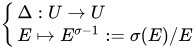
彼は、拡大体の 単位群の2つの自己準同型性を、 群 に関する ガロア加群 、簡単に言えば -加群として考察した。最初の自己準同型性は
U
=
U
L
{\displaystyle U=U_{L}}
G
{\displaystyle G}
G
{\displaystyle G}
{
Δ
:
U
→
U
E
↦
E
σ
−
1
:=
σ
(
E
)
/
E
{\displaystyle {\begin{cases}\Delta :U\to U\\E\mapsto E^{\sigma -1}:=\sigma (E)/E\end{cases}}}
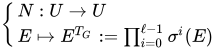
は差を持つシンボリック累乗であり 、第二準同型性
σ
−
1
∈
Z
[
G
]
{\displaystyle \sigma -1\in \mathbb {Z} [G]}
{
N
:
U
→
U
E
↦
E
T
G
:=
∏
i
=
0
ℓ
−
1
σ
i
(
E
)
{\displaystyle {\begin{cases}N:U\to U\\E\mapsto E^{T_{G}}:=\prod _{i=0}^{\ell -1}\sigma ^{i}(E)\end{cases}}}
は 代数的ノルム 写像、つまりトレース
T
G
=
∑
i
=
0
ℓ
−
1
σ
i
∈
Z
[
G
]
.
{\displaystyle T_{G}=\sum _{i=0}^{\ell -1}\sigma ^{i}\in \mathbb {Z} [G].}
実際、代数ノルム写像の像は 基底体の単位群に含まれており、すべての共役の積としての 通常の 算術(体)ノルム と一致します。自己準同型の合成は、関係 とを満たします 。
U
K
{\displaystyle U_{K}}
N
(
E
)
=
N
L
/
K
(
E
)
{\displaystyle N(E)=\mathrm {N} _{L/K}(E)}
Δ
∘
N
=
1
{\displaystyle \Delta \circ N=1}
N
∘
Δ
=
1
{\displaystyle N\circ \Delta =1}
これらの自己準同型の核と像を用いて、2 つの重要なコホモロジー群を定義できます。 における のゼロ次 テイトコホモロジー群は 、の ノルム留数 からなる 商で与えられ、 における のマイナス 1 次テイトコホモロジー群は、形式指数 を持つ単位 の 記号的冪の部分群 を法とする の 相対単位 群の 商で与えられます 。
G
{\displaystyle G}
U
L
{\displaystyle U_{L}}
H
0
(
G
,
U
L
)
:=
ker
(
Δ
)
/
i
m
(
N
)
=
U
K
/
N
L
/
K
(
U
L
)
{\displaystyle H^{0}(G,U_{L}):=\ker(\Delta )/\mathrm {im} (N)=U_{K}/\mathrm {N} _{L/K}(U_{L})}
U
K
{\displaystyle U_{K}}
G
{\displaystyle G}
U
L
{\displaystyle U_{L}}
H
−
1
(
G
,
U
L
)
:=
ker
(
N
)
/
i
m
(
Δ
)
=
E
L
/
K
/
U
L
σ
−
1
{\displaystyle H^{-1}(G,U_{L}):=\ker(N)/\mathrm {im} (\Delta )=E_{L/K}/U_{L}^{\sigma -1}}
E
L
/
K
=
{
E
∈
U
L
|
N
(
E
)
=
1
}
{\displaystyle E_{L/K}=\{E\in U_{L}|N(E)=1\}}
L
/
K
{\displaystyle L/K}
σ
−
1
{\displaystyle \sigma -1}
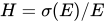
ヒルベルトは定理92 で、 任意の単位 に対して として表すことができない 相対単位 の存在を証明しています。これは、マイナス第一コホモロジー群 が で 割り切れる位の非自明である ことを意味します 。しかし、完全に同様の構成の助けを借りて、 超体 の乗法群である -加群のマイナス第一コホモロジー群 を定義することができ、ヒルベルトは有名な 定理90 でその自明性を示しています 。
H
∈
E
L
/
K
{\displaystyle H\in E_{L/K}}
H
=
σ
(
E
)
/
E
{\displaystyle H=\sigma (E)/E}
E
∈
U
L
{\displaystyle E\in U_{L}}
H
−
1
(
G
,
U
L
)
=
E
L
/
K
/
U
L
σ
−
1
{\displaystyle H^{-1}(G,U_{L})=E_{L/K}/U_{L}^{\sigma -1}}
ℓ
{\displaystyle \ell }
H
−
1
(
G
,
L
×
)
=
{
A
∈
L
×
|
N
(
A
)
=
1
}
/
(
L
×
)
σ
−
1
{\displaystyle H^{-1}(G,L^{\times })=\{A\in L^{\times }|N(A)=1\}/(L^{\times })^{\sigma -1}}
G
{\displaystyle G}
L
×
=
L
∖
{
0
}
{\displaystyle L^{\times }=L\setminus \{0\}}
L
{\displaystyle L}
H
−
1
(
G
,
L
×
)
=
1
{\displaystyle H^{-1}(G,L^{\times })=1}
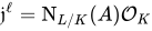
最終的に、ヒルベルトは有名な定理94を 述べる立場になります 。が、 自明な相対判別式 を持つ 奇数素数次数体の巡回拡大である場合 、つまり 有限素数 で非分岐である場合、拡大体 において主となる、 基底体の 非主イデアルが存在し 、これは に対して存在します 。さらに、 この非主イデアルの 番目の乗は 、特に基底体 において主である ため、基底体の類数は で割り切れる必要があり 、拡大体は の 類体 と呼ぶことができます 。証明は以下のとおりです。定理92は単位 が存在することを述べており、定理90は となる (必然的に非単位) の存在を保証します。 つまり です。必要であれば適切な整数を 乗じることで、は 代数 的整数であると 仮定 でき ます 。しかし、 部分体の 根底にあるイデアルは 主イデアルにはなり得ません。逆に、 何らかの に対してであると仮定します 。 は非分岐なので、 の あらゆる曖昧なイデアルは 、特に における何らかのイデアルの持ち上げです 。したがって 、 何らかの単位 に対してとなります。これは のため、 矛盾を意味します 。一方、
L
/
K
{\displaystyle L/K}
ℓ
{\displaystyle \ell }
d
L
/
K
=
O
K
{\displaystyle {\mathfrak {d}}_{L/K}={\mathcal {O}}_{K}}
j
∈
I
K
∖
P
K
{\displaystyle {\mathfrak {j}}\in {\mathcal {I}}_{K}\setminus {\mathcal {P}}_{K}}
K
{\displaystyle K}
L
{\displaystyle L}
j
O
L
=
A
O
L
∈
P
L
{\displaystyle {\mathfrak {j}}{\mathcal {O}}_{L}=A{\mathcal {O}}_{L}\in {\mathcal {P}}_{L}}
A
∈
O
L
{\displaystyle A\in {\mathcal {O}}_{L}}
ℓ
{\displaystyle \ell }
K
{\displaystyle K}
j
ℓ
=
N
L
/
K
(
A
)
O
K
∈
P
K
{\displaystyle {\mathfrak {j}}^{\ell }=\mathrm {N} _{L/K}(A){\mathcal {O}}_{K}\in {\mathcal {P}}_{K}}
ℓ
{\displaystyle \ell }
L
{\displaystyle L}
K
{\displaystyle K}
H
∈
E
L
/
K
∖
U
L
σ
−
1
{\displaystyle H\in E_{L/K}\setminus U_{L}^{\sigma -1}}
A
∈
L
×
{\displaystyle A\in L^{\times }}
H
=
A
σ
−
1
{\displaystyle H=A^{\sigma -1}}
A
σ
=
A
⋅
H
{\displaystyle A^{\sigma }=A\cdot H}
A
{\displaystyle A}
A
{\displaystyle A}
A
{\displaystyle A}
L
/
K
{\displaystyle L/K}
(
A
O
L
)
σ
=
A
σ
O
L
=
A
⋅
H
O
L
=
A
O
L
{\displaystyle (A{\mathcal {O}}_{L})^{\sigma }=A^{\sigma }{\mathcal {O}}_{L}=A\cdot H{\mathcal {O}}_{L}=A{\mathcal {O}}_{L}}
j
:=
(
A
O
L
)
∩
O
K
{\displaystyle {\mathfrak {j}}:=(A{\mathcal {O}}_{L})\cap {\mathcal {O}}_{K}}
K
{\displaystyle K}
j
=
β
O
K
{\displaystyle {\mathfrak {j}}=\beta {\mathcal {O}}_{K}}
β
∈
O
K
{\displaystyle \beta \in {\mathcal {O}}_{K}}
L
/
K
{\displaystyle L/K}
a
{\displaystyle {\mathfrak {a}}}
O
L
{\displaystyle {\mathcal {O}}_{L}}
O
K
{\displaystyle {\mathcal {O}}_{K}}
a
=
(
a
∩
O
K
)
O
L
{\displaystyle {\mathfrak {a}}=({\mathfrak {a}}\cap {\mathcal {O}}_{K}){\mathcal {O}}_{L}}
β
O
L
=
j
O
L
=
A
O
L
{\displaystyle \beta {\mathcal {O}}_{L}={\mathfrak {j}}{\mathcal {O}}_{L}=A{\mathcal {O}}_{L}}
A
=
β
E
{\displaystyle A=\beta E}
E
∈
U
L
{\displaystyle E\in U_{L}}
H
=
A
σ
−
1
=
(
β
E
)
σ
−
1
=
E
σ
−
1
{\displaystyle H=A^{\sigma -1}=(\beta E)^{\sigma -1}=E^{\sigma -1}}
β
σ
−
1
=
1
{\displaystyle \beta ^{\sigma -1}=1}
j
ℓ
O
L
=
(
j
O
L
)
ℓ
=
N
L
/
K
(
j
O
L
)
O
L
=
N
L
/
K
(
A
O
L
)
O
L
=
N
L
/
K
(
A
)
O
L
,
{\displaystyle {\mathfrak {j}}^{\ell }{\mathcal {O}}_{L}=({\mathfrak {j}}{\mathcal {O}}_{L})^{\ell }=\mathrm {N} _{L/K}({\mathfrak {j}}{\mathcal {O}}_{L}){\mathcal {O}}_{L}=\mathrm {N} _{L/K}(A{\mathcal {O}}_{L}){\mathcal {O}}_{L}=\mathrm {N} _{L/K}(A){\mathcal {O}}_{L},}
したがって、 ベース フィールドでは すでにプリンシパルになっています。
j
ℓ
=
N
L
/
K
(
A
)
O
K
{\displaystyle {\mathfrak {j}}^{\ell }=\mathrm {N} _{L/K}(A){\mathcal {O}}_{K}}
K
{\displaystyle K}
定理 92 と 94 は、体とが 反例である状態で、 については述べられているようには成り立ちません (この特定のケースでは、 の 狭い ヒルベルト 類体 です )。その理由は、ヒルベルトは有限素数での分岐のみを考慮し、無限素数での分岐は考慮しないからです ( の実無限素数が に分岐するのは 、この素数の への非実数拡張が存在する場合です )。 が奇数のときは、拡張が無限素数で非分岐になるため、これは違いを生じません。しかし、 に共役な実体の数が に 共役な実体の数の 2 倍であるとさらに 仮定すれば、定理 92 と 94 が について成立することを彼は指摘しています。 この条件は、無限素数で非分岐であることと同等であるため、 が どこでも非分岐である
と仮定すれば、 定理 94 はすべての素数について成立します。
ℓ
=
2
{\displaystyle \ell =2}
K
=
Q
(
3
)
{\displaystyle K=\mathbb {Q} ({\sqrt {3}})}
L
=
K
(
i
)
{\displaystyle L=K(i)}
L
{\displaystyle L}
K
{\displaystyle K}
K
{\displaystyle K}
L
{\displaystyle L}
L
{\displaystyle L}
[
L
:
K
]
{\displaystyle [L:K]}
ℓ
=
2
{\displaystyle \ell =2}
L
{\displaystyle L}
K
{\displaystyle K}
L
/
K
{\displaystyle L/K}
ℓ
{\displaystyle \ell }
L
/
K
{\displaystyle L/K}
定理94は、拡大 の主核の位数に関する 単純な不等式を示唆している 。しかし、この核の位数の正確な公式は、巡回非分岐(無限素数を含む)拡大(必ずしも素数次ではない)に対して、 - 加群 の エルブラン商 [11] を用いて導くことができ、それは次のように与えられる。
#
ker
(
j
L
/
K
)
≥
ℓ
=
[
L
:
K
]
{\displaystyle \#\ker(j_{L/K})\geq \ell =[L:K]}
L
/
K
{\displaystyle L/K}
h
(
G
,
U
L
)
{\displaystyle h(G,U_{L})}
G
{\displaystyle G}
U
L
{\displaystyle U_{L}}
h
(
G
,
U
L
)
:=
#
H
−
1
(
G
,
U
L
)
/
#
H
0
(
G
,
U
L
)
=
(
ker
(
N
)
:
i
m
(
Δ
)
)
/
(
ker
(
Δ
)
:
i
m
(
N
)
)
=
(
E
L
/
K
:
U
L
σ
−
1
)
/
(
U
K
:
N
L
/
K
(
U
L
)
)
.
{\displaystyle h(G,U_{L}):=\#H^{-1}(G,U_{L})/\#H^{0}(G,U_{L})=(\ker(N):\mathrm {im} (\Delta ))/(\ker(\Delta ):\mathrm {im} (N))=(E_{L/K}:U_{L}^{\sigma -1})/(U_{K}:\mathrm {N} _{L/K}(U_{L})).}
(どちらのコホモロジー群の順序も計算せずに) が示される。拡大は 非分岐なので、 となる。 長さ の周期コホモロジーを持つ巡回拡大に特化したK. Iwasawa の同型 [12] の助けを借りて、次 を得る。
h
(
G
,
U
L
)
=
[
L
:
K
]
{\displaystyle h(G,U_{L})=[L:K]}
L
/
K
{\displaystyle L/K}
I
L
G
=
I
K
O
L
{\displaystyle {\mathcal {I}}_{L}^{G}={\mathcal {I}}_{K}{\mathcal {O}}_{L}}
P
L
G
=
P
L
∩
I
K
O
L
{\displaystyle {\mathcal {P}}_{L}^{G}={\mathcal {P}}_{L}\cap {\mathcal {I}}_{K}{\mathcal {O}}_{L}}
H
1
(
G
,
U
L
)
≅
P
L
G
/
P
K
O
L
{\displaystyle H^{1}(G,U_{L})\cong {\mathcal {P}}_{L}^{G}/{\mathcal {P}}_{K}{\mathcal {O}}_{L}}
2
{\displaystyle 2}
#
ker
(
j
L
/
K
)
=
#
(
P
L
∩
I
K
O
L
/
P
K
O
L
)
=
#
(
P
L
G
/
P
K
O
L
)
=
#
H
1
(
G
,
U
L
)
=
#
H
−
1
(
G
,
U
L
)
=
h
(
G
,
U
L
)
⋅
#
H
0
(
G
,
U
L
)
=
[
L
:
K
]
⋅
#
H
0
(
G
,
U
L
)
=
[
L
:
K
]
⋅
(
U
K
:
N
L
/
K
(
U
L
)
)
{\displaystyle {\begin{aligned}\#\ker(j_{L/K})&=\#({\mathcal {P}}_{L}\cap {\mathcal {I}}_{K}{\mathcal {O}}_{L}/{\mathcal {P}}_{K}{\mathcal {O}}_{L})=\#({\mathcal {P}}_{L}^{G}/{\mathcal {P}}_{K}{\mathcal {O}}_{L})=\#H^{1}(G,U_{L})=\#H^{-1}(G,U_{L})\\&=h(G,U_{L})\cdot \#H^{0}(G,U_{L})=[L:K]\cdot \#H^{0}(G,U_{L})=[L:K]\cdot (U_{K}:\mathrm {N} _{L/K}(U_{L}))\end{aligned}}}
この関係により、下限が係数 、いわゆる 単位ノルム指数 だけ増加します。
(
U
K
:
N
L
/
K
(
U
L
)
)
{\displaystyle (U_{K}:\mathrm {N} _{L/K}(U_{L}))}
歴史 リードセクションで述べたように、1930 年のヒルベルト-アルティン-フルトヴェングラー主イデアル定理を、基底体とそのヒルベルト類体との間の中間拡大における主化に関する問題に一般化しようとした研究者が何人かいた。一方では、Ph. Furtwängler 1932、 [13]
O. Taussky 1932、 [14]
O. Taussky 1970、 [15]
および H. Kisilevsky 1970 [16] など、任意の数体
上の主化に関する一般定理を確立した。他方では、特定の種類の基底体の非分岐巡回拡大における主化の具体的な数値例を探した。
二次方程式 非分岐巡回 三次拡大における - 類階数 2 の虚数二次体 の - 類 の主化は、1934 年に A. Scholz と O. Taussky [7] によって 3 つの判別式に対して手動で計算されました
。これらの計算には、2 進二次形式の合成と三次数体の基本単位系の明示的な知識が必要であり、これは 1934 年当時は非常に困難な作業であったため、調査は半世紀の間停滞していましたが、1982 年に F.-P. Heider と B. Schmithals [17]
がケルン大学の CDC Cyber 76 コンピュータを使用して、主化に関する情報を関連する判別式 を含む範囲に拡張し 、5 つの実二次体の最初の解析を提供しました。2 年後、JR Brink [18] は複素二次体
の主化タイプを計算しました。現在、判別式 と 型のクラス群 を持つすべての二次体 に対するプリンシパル化データの最も広範な計算は 、2010年のDC Mayerによるものであり、 [19]彼は、転送カーネルと転送ターゲットの間に最近発見された関係を使用して、新しい プリンシパル化アルゴリズム
を設計しました 。 [20]
3
{\displaystyle 3}
K
=
Q
(
d
)
{\displaystyle K=\mathbb {Q} ({\sqrt {d}})}
3
{\displaystyle 3}
d
∈
{
−
3299
,
−
4027
,
−
9748
}
{\displaystyle d\in \{-3299,-4027,-9748\}}
−
2
⋅
10
4
<
d
<
10
5
{\displaystyle -2\cdot 10^{4}<d<10^{5}}
27
{\displaystyle 27}
66
{\displaystyle 66}
4596
{\displaystyle 4596}
−
10
6
<
d
<
10
7
{\displaystyle -10^{6}<d<10^{7}}
3
{\displaystyle 3}
(
3
,
3
)
{\displaystyle (3,3)}
型の -クラス群 を持つ虚二次体の非分岐二次拡大における -主化は、 1976 年にH. Kisilevskyによって研究されました。 [21]
実二次体に関する同様の研究は、1995年にE. BenjaminとC. Snyderによって行われました。 [22]
2
{\displaystyle 2}
2
{\displaystyle 2}
(
2
,
2
)
{\displaystyle (2,2)}
立方体フィールド 型の -クラス群 を 持つ巡回3 次体 の非分岐2次拡大における -主化は、 1988 年にA. Derhemによって研究されました。 [23]
7年後、M. Ayadiは、 型の -クラス群 と2つまたは3つの素数で割り切れる導体 を持つ巡回3次体 、 の非分岐巡回3次拡大における- 主化を研究しました。 [24]
2
{\displaystyle 2}
2
{\displaystyle 2}
(
2
,
2
)
{\displaystyle (2,2)}
3
{\displaystyle 3}
K
⊂
Q
(
ζ
f
)
{\displaystyle K\subset \mathbb {Q} (\zeta _{f})}
ζ
f
f
=
1
{\displaystyle \zeta _{f}^{f}=1}
3
{\displaystyle 3}
(
3
,
3
)
{\displaystyle (3,3)}
f
{\displaystyle f}
六次フィールド 1992年に、MC Ismailiは、この六次数体 、が 型の -クラス群 を持つ 場合、 純粋な3次体 の 正規 閉包 の非分岐巡回3次拡大における -主化を調査しました 。 [25]
3
{\displaystyle 3}
K
=
Q
(
D
3
)
{\displaystyle K=\mathbb {Q} ({\sqrt[{3}]{D}})}
N
=
K
(
ζ
3
)
{\displaystyle N=K(\zeta _{3})}
ζ
3
3
=
1
{\displaystyle \zeta _{3}^{3}=1}
3
{\displaystyle 3}
(
3
,
3
)
{\displaystyle (3,3)}
四次フィールド 1993 年、A. Azizi は、型の - 類群を持つディリクレ型の双四次体の非分岐二次拡大における - 主化を研究しました 。[26] 最近では、2014 年に A. Zekhnini が、型の - 類群を持つディリクレ体に調査を拡張し、[27] ランク 3 の類群を 持つ 四 次 体 の 非 分岐 二 次 拡大 と 双四次拡大の 2 層における - 主化 の最初の例を示しました 。
2
{\displaystyle 2}
K
=
Q
(
d
,
−
1
)
{\displaystyle K=\mathbb {Q} ({\sqrt {d}},{\sqrt {-1}})}
2
{\displaystyle 2}
(
2
,
2
)
{\displaystyle (2,2)}
2
{\displaystyle 2}
(
2
,
2
,
2
)
{\displaystyle (2,2,2)}
2
{\displaystyle 2}
2
{\displaystyle 2}
参照 ヒルベルト=アルティン=フルトヴェングラーによる代数的、群論的アプローチとヒルベルト=ヘルブラント=岩澤による算術的、コホモロジー的アプローチは、 J.-F. ヤウレント 1988 [28] と K. ミヤケ 1989 [6]による 2 つの 降伏のバイブルでも詳細に紹介されている。
二次資料 Cassels, JWS ; Fröhlich, Albrecht 編 (1967). 代数的数論 . Academic Press. Zbl 0153.07403. 岩沢健吉 (1986)。 局所類体理論。オックスフォード数学モノグラフ 。 オックスフォード大学出版局。ISBN 978-0-19-504030-2 . MR 0863740. Zbl 0604.12014. Janusz, Gerald J. (1973). 代数的数体 . 純粋および応用数学. 第55巻. Academic Press. p. 142. Zbl 0307.12001. ノイキルヒ、ユルゲン (1999)。 代数的整数論 。 Grundlehren der Mathematischen Wissenschaften。 Vol. 322. シュプリンガー・ フェルラーグ ISBN 978-3-540-65399-8 . MR 1697859. Zbl 0956.11021. Neukirch, ユルゲン ;シュミット、アレクサンダー。ウィンバーグ、ケイ (2008)。 数体のコホモロジー 。 Grundlehren der Mathematischen Wissenschaften (ドイツ語)。 Vol. 323 (第 2 版)。 スプリンガー・フェルラーグ 。 ISBN 978-3-540-37888-4 .ZBL1136.11001 。
参考文献
^ ハーヴィッツ、A. (1926)。 「Über Beziehungen zwischen den Primidealen eines algebraischen Körpers und den Substitutionen seiner Gruppe」。 数学。 Z. (ドイツ語)。 25 : 661–665。 土井 :10.1007/bf01283860。 S2CID 119971823。 ^ ab ヒルベルト、D. (1897)。 「代数理論に関するZahlkörper」。 ヤーレスベル。ドイツ語。数学。ヴェライン。 (ドイツ語で)。 4 : 175–546。 ^ ab Hasse、H. (1930)。 「Bericht über neuere Untersuhungen und Probleme aus der Theorie der algebraischen Zahlkörper. Teil II: Reziprozitätsgesetz」。 ヤーレスベル。ドイツ語。数学。 Verein.、Ergänzungsband (ドイツ語)。 6 :1~204。
^ アーティン、E. (1927)。 「Beweis des allgemeinen Reziprozitätsgesetzes」。 ああ。数学。セム。大学ハンブルク (ドイツ語)。 5 : 353–363。 土井 :10.1007/BF02952531。 S2CID 123050778。
^ アーティン、E. (1929)。 「オーバーコルペルンとアルゲマイネスの理想的なクラッセン」。 ああ。数学。セム。大学ハンブルク (ドイツ語)。 7 : 46–51。 土井 :10.1007/BF02941159。 S2CID 121475651。
^ ab Miyake, K. (1989). 「ヒルベルトの定理94、主イデアル定理、および降伏問題の代数的研究」. Expo. Math . 7 : 289–346.
^ ab ショルツ、A.、タウスキー、O. (1934)。 「Die Hauptideale der kubischen Klassenkörper imaginär quadratischer Zahlkörper: ihre rechnerische Bestimmung und ihr Einfluß auf den Klassenkörperturm」。 J. レーヌ・アンジェウ数学。 (ドイツ語で)。 171 :19-41。
{{cite journal}}: CS1 maint: multiple names: authors list (link)
^ シュライヤー、O. (1926)。 「グルッペン II 世の統治者」。 ああ。数学。セム。大学ハンブルク (ドイツ語)。 4 : 321–346。 土井 :10.1007/BF02950735。 S2CID 122947636。
^ Newman, MF (1977). 素数冪順序の群の決定 。pp. 73-84、Group Theory、キャンベラ、1975年、Lecture Notes in Math.、Vol. 573、Springer、ベルリン。
^ O'Brien, EA (1990). 「pグループ生成アルゴリズム」 J. Symbolic Comput . 9 (5–6): 677–698. doi : 10.1016/s0747-7171(08)80082-x .
^ Herbrand、J. (1932)。 「ジャンルの主要な原理と原理的な原理」。 ああ。数学。セム。大学ハンブルク (フランス語)。 9 : 84–92。 土井 :10.1007/bf02940630。 S2CID 120775483。 ^ 岩沢 憲一 (1956). 「代数体の単位群に関するノート」 J. Math. Pures Appl . 9 (35): 189–192.
^ フルトヴェングラー博士 (1932)。 「代数Zahlkörperの最適な機能」。 J. レーヌ・アンジェウ数学。 (ドイツ語で)。 1932 (167): 379–387。 土井 :10.1515/crll.1932.167.379。 S2CID 199546266。
^ タウスキー、O. (1932)。 「代数Zahlkörperの最適な機能」。 J. レーヌ・アンジェウ数学。 (ドイツ語で)。 1932 (168): 193–210。 土井 :10.1515/crll.1932.168.193。 S2CID 199545623。
^ Taussky, O. (1970). 「ヒルベルトの定理94に関するコメント」 J. Reine Angew. 数学 . 239/240: 435–438.
^ Kisilevsky, H. (1970). 「ヒルベルトの定理94に関連するいくつかの結果」. J. Number Theory . 2 (2): 199–206. Bibcode :1970JNT.....2..199K. doi : 10.1016/0022-314x(70)90020-x .
^ ハイダー、F.-P.、シュミタールス、B. (1982)。 「Zur Kapitulation der Idealklassen in unverzweigten primzyklischen Erweiterungen」。 J. レーヌ・アンジェウ数学。 (ドイツ語で)。 363 : 1-25.
{{cite journal}}: CS1 maint: multiple names: authors list (link)
^ Brink, JR (1984). 型 (3,3) の虚二次数体の類体タワー 。オハイオ州立大学博士論文。
^ Mayer, DC (2012). 「数体の第2pクラス群」. Int. J. Number Theory . 8 (2): 471–505. arXiv : 1403.3899 . doi :10.1142/s179304211250025x. S2CID 119332361.
^ Mayer, DC (2014). 「クラスグループ構造によるプリンシパル化アルゴリズム」 J. Théor. Nombres Bordeaux . 26 (2): 415–464. arXiv : 1403.3839 . doi :10.5802/jtnb.874. S2CID 119740132.
^ Kisilevsky, H. (1976). 「4 mod 8に合同な類数を持つ数体とヒルベルトの定理94」. J. Number Theory . 8 (3): 271–279. doi : 10.1016/0022-314x(76)90004-4 .
^ Benjamin, E., Snyder, C. (1995). 「(2,2) 型の 2 クラス群を持つ実二次数体」. Math. Scand . 76 : 161–178. doi : 10.7146/math.scand.a-12532 .
{{cite journal}}: CS1 maint: multiple names: authors list (link)
^ A. ダーヘム (1988)。 Capitulation dans les extensions quadratiques non ramifiées de corps de nombres cubiques cycliques (フランス語)。テーゼ・ド・ドクター、Univ.ケベック州ラヴァル。
^ アヤディ、M. (1995)。 Sur la capitulation de 3-classes d'idéaux d'un corps cubique cyclique (フランス語)。テーゼ・ド・ドクター、Univ.ケベック州ラヴァル。
^ イスマーイリ、MC (1992)。 Sur la capitulation de 3-classes d'idéaux de la clôture Normale d'un corps cubique pure (フランス語)。テーゼ・ド・ドクター、Univ.ケベック州ラヴァル。
^ アジジ、A. (1993)。 Sur la capitulation de 2-classes d'idéaux de (フランス語)。テーゼ・ド・ドクター、Univ.ケベック州ラヴァル。
Q
(
d
,
i
)
{\displaystyle \mathbb {Q} ({\sqrt {d}},i)}
^ Zekhnini、A. (2014)。 Capitulation des 2-classes d'idéaux de specifics corps de nombres biquadratiques imaginaires de type (2,2,2) (フランス語)。テーゼ・ド・ドクター、Univ.モロッコ、ウジダ科学学部のモハメッド・プレミア。
Q
(
d
,
i
)
{\displaystyle \mathbb {Q} ({\sqrt {d}},i)}
^ ジャウレント、J.-F. (1988年2月26日)。 「降伏の問題の現実」。 Séminaire de Théorie des Nombres de Bordeaux (フランス語)。 17 :1-33。






























![{\textstyle \left[{\frac {F/K}{\mathfrak {P}}}\right]:=\sigma }](https://wikimedia.org/api/rest_v1/media/math/render/svg/818f90920d7bee7fddb993b71980767b3b629710)


![{\displaystyle f:=f({\mathfrak {P}}|{\mathfrak {p}})=[{\mathcal {O}}_{F}/{\mathfrak {P}}:{\mathcal {O}}_{K}/{\mathfrak {p}}]}](https://wikimedia.org/api/rest_v1/media/math/render/svg/ae4e8576a122c7a7892c75c4567f08f854de5142)
![{\textstyle \left[{\frac {F/K}{\mathfrak {P}}}\right]}](https://wikimedia.org/api/rest_v1/media/math/render/svg/6beebae277927d705c597fe35d2017d5b0b2a73a)




![{\displaystyle \left[{\frac {F/K}{\tau ({\mathfrak {P}})}}\right]=\tau \left[{\frac {F/K}{\mathfrak {P}}}\right]\tau ^{-1},}](https://wikimedia.org/api/rest_v1/media/math/render/svg/b6f61c9b25d97c3b213cf0ea5e30941118433ecf)

![{\displaystyle {\mathfrak {p}}\mapsto \left({\frac {F/K}{\mathfrak {p}}}\right):=\left.\left\{\tau \left[{\frac {F/K}{\mathfrak {P}}}\right]\tau ^{-1}\right|\tau \in G\right\}}](https://wikimedia.org/api/rest_v1/media/math/render/svg/fbd84d61cd28fd4aa567b23f4642c7240fe22cf4)























![{\textstyle \left({\frac {F/K}{\mathfrak {p}}}\right)=\left[{\frac {F/K}{\mathfrak {P}}}\right]}](https://wikimedia.org/api/rest_v1/media/math/render/svg/538e82ce1c040b3479cf85038f22be2c1428ce1c)



























![{\displaystyle \prod _{i=1}^{g}\left({\frac {L'/L}{{\mathfrak {q}}_{i}}}\right)=\prod _{i=1}^{g}\left[{\frac {F/L}{\tau _{i}({\mathfrak {P}})}}\right]\cdot H'=\prod _{i=1}^{g}\tau _{i}\left[{\frac {F/L}{\mathfrak {P}}}\right]\tau _{i}^{-1}\cdot H'=\prod _{i=1}^{g}\tau _{i}\left[{\frac {F/K}{\mathfrak {P}}}\right]^{f_{i}}\tau _{i}^{-1}\cdot H',}](https://wikimedia.org/api/rest_v1/media/math/render/svg/beb6936783b391c014f46aa835eed4508ccafa08)

![{\textstyle \left({\frac {K'/K}{\mathfrak {p}}}\right)=\left[{\frac {F/K}{\mathfrak {P}}}\right]\cdot G'}](https://wikimedia.org/api/rest_v1/media/math/render/svg/b613c3a3bbfefc8b47e1544b134e6dcdf90f554c)



![{\textstyle \left[{\frac {F/K}{\mathfrak {P}}}\right]\cdot G'}](https://wikimedia.org/api/rest_v1/media/math/render/svg/36d58a463c576db36edfedb822346e6df6e300d8)
![{\displaystyle {\tilde {T}}_{G,H}\left(\left[{\frac {F/K}{\mathfrak {P}}}\right]\cdot G'\right)=T_{G,H}\left(\left[{\frac {F/K}{\mathfrak {P}}}\right]\right)=\prod _{i=1}^{g}(\tau _{i}^{-1})^{-1}\left[{\frac {F/K}{\mathfrak {P}}}\right]^{f_{i}}\tau _{i}^{-1}\cdot H'=\prod _{i=1}^{g}\tau _{i}\left[{\frac {F/K}{\mathfrak {P}}}\right]^{f_{i}}\tau _{i}^{-1}\cdot H'.}](https://wikimedia.org/api/rest_v1/media/math/render/svg/78f49003c89e0dce98352e1d054f68d6923e8d25)










![{\displaystyle [G:G']<\infty }](https://wikimedia.org/api/rest_v1/media/math/render/svg/946d6ccd5234f0d21d7d3ae5bd93e8e500225fab)








![{\displaystyle \ell =[L:K]}](https://wikimedia.org/api/rest_v1/media/math/render/svg/7c4b21978bcb9cd321993ad861c71bd5a9e60ff7)

![{\displaystyle \sigma -1\in \mathbb {Z} [G]}](https://wikimedia.org/api/rest_v1/media/math/render/svg/56a10abbe607e19db98567ab7e5377a121e9f29f)
![{\displaystyle T_{G}=\sum _{i=0}^{\ell -1}\sigma ^{i}\in \mathbb {Z} [G].}](https://wikimedia.org/api/rest_v1/media/math/render/svg/8a6ae10759414d801c703807bb97ad767afc66ba)
































![{\displaystyle [L:K]}](https://wikimedia.org/api/rest_v1/media/math/render/svg/aece5b0ecef53af76d4af496d68ed1c41532bb79)
![{\displaystyle \#\ker(j_{L/K})\geq \ell =[L:K]}](https://wikimedia.org/api/rest_v1/media/math/render/svg/789fc9cfaaf813d91fe1db8f38c056ac44d235fc)


![{\displaystyle h(G,U_{L})=[L:K]}](https://wikimedia.org/api/rest_v1/media/math/render/svg/657db722bdeb32595a65aa1364a9401dd26396a7)




![{\displaystyle {\begin{aligned}\#\ker(j_{L/K})&=\#({\mathcal {P}}_{L}\cap {\mathcal {I}}_{K}{\mathcal {O}}_{L}/{\mathcal {P}}_{K}{\mathcal {O}}_{L})=\#({\mathcal {P}}_{L}^{G}/{\mathcal {P}}_{K}{\mathcal {O}}_{L})=\#H^{1}(G,U_{L})=\#H^{-1}(G,U_{L})\\&=h(G,U_{L})\cdot \#H^{0}(G,U_{L})=[L:K]\cdot \#H^{0}(G,U_{L})=[L:K]\cdot (U_{K}:\mathrm {N} _{L/K}(U_{L}))\end{aligned}}}](https://wikimedia.org/api/rest_v1/media/math/render/svg/116cdc33cfdc3f3bbee39cfd9b46ab2b1380f605)










![{\displaystyle K=\mathbb {Q} ({\sqrt[{3}]{D}})}](https://wikimedia.org/api/rest_v1/media/math/render/svg/50f2fa5fbd5725a45d39e412f89b89488ad20c7f)




