無限次元の例 無限次元における最も単純な(非自明な)例の1つは、領域がヒルベルト空間 である場合である(H {\displaystyle H} ‖ ⋅ ‖ : H → R 。 {\displaystyle \|\,\cdot \,\|:H\to \mathbb {R} .}
まず、x ≠ 0. {\displaystyle x\neq 0.} ‖ ⋅ ‖ {\displaystyle \|\cdot \|} x {\displaystyle x} D 、 {\displaystyle D,} D v := ⟨ x ‖ x ‖ 、 v ⟩ 。 {\displaystyle Dv:=\left\langle {\frac {x}{\|x\|}},v\right\rangle .}
確かに、 | ‖ x + h ‖ − ‖ x ‖ − D h | ‖ h ‖ = | ‖ x ‖ ‖ x + h ‖ − ⟨ x 、 x ⟩ − ⟨ x 、 h ⟩ | ‖ x ‖ ‖ h ‖ = | ‖ x ‖ ‖ x + h ‖ − ⟨ x 、 x + h ⟩ | ‖ x ‖ ‖ h ‖ = | ⟨ x 、 x ⟩ ⟨ x + h 、 x + h ⟩ − ⟨ x 、 x + h ⟩ 2 | ‖ x ‖ ‖ h ‖ ( | ‖ x ‖ ‖ x + h ‖ + ⟨ x 、 x + h ⟩ | ) = ⟨ x 、 x ⟩ ⟨ h 、 h ⟩ − ⟨ x 、 h ⟩ 2 ‖ x ‖ ‖ h ‖ ( | ‖ x ‖ ‖ x + h ‖ + ⟨ x 、 x + h ⟩ | ) {\displaystyle {\begin{aligned}{\frac {|\|x+h\|-\|x\|-Dh|}{\|h\|}}&={\frac {|\|x\|\|x+h\|-\langle x,x\rangle -\langle x,h\rangle |}{\|x\|\|h\|}}\\[8pt]&={\frac {|\|x\|\|x+h\|-\langle x,x+h\rangle |}{\|x\|\|h\|}}\\[8pt]&={\frac {|\langle x,x\rangle \langle x+h,x+h\rangle -\langle x,x+h\rangle ^{2}|}{\|x\|\|h\|(|\|x\|\|x+h\|+\langle x,x+h\rangle |)}}\\[8pt]&={\frac {\langle x,x\rangle \langle h,h\rangle -\langle x,h\rangle ^{2}}{\|x\|\|h\|(|\|x\|\|x+h\|+\langle x,x+h\rangle |)}}\\&{}\end{aligned}}}
ノルムの連続性と内積を用いると、次の式が得られます。 リム ‖ h ‖ → 0 | ‖ x + h ‖ − ‖ x ‖ − D h | ‖ h ‖ = リム ‖ h ‖ → 0 ⟨ x 、 x ⟩ ⟨ h 、 h ⟩ − ⟨ x 、 h ⟩ 2 ‖ x ‖ ‖ h ‖ ( | ‖ x ‖ ‖ x + h ‖ + ⟨ x 、 x + h ⟩ | ) = 1 2 ‖ x ‖ 3 リム ‖ h ‖ → 0 ⟨ x 、 x ⟩ ⟨ h 、 h ⟩ − ⟨ x 、 h ⟩ 2 ‖ h ‖ = 1 2 ‖ x ‖ 3 リム ‖ h ‖ → 0 ( ⟨ x 、 x ⟩ ‖ h ‖ − ⟨ x 、 h ⟩ ⟨ x 、 h ‖ h ‖ ⟩ ) = 1 2 ‖ x ‖ 3 ( リム ‖ h ‖ → 0 ⟨ x 、 x ⟩ ‖ h ‖ − リム h → 0 ⟨ x 、 h ⟩ ⟨ x 、 h ‖ h ‖ ⟩ ) = 1 2 ‖ x ‖ 3 ( 0 − リム ‖ h ‖ → 0 ⟨ x 、 h ⟩ ⟨ x 、 h ‖ h ‖ ⟩ ) = − 1 2 ‖ x ‖ 3 ( リム ‖ h ‖ → 0 ⟨ x 、 h ⟩ ⟨ x 、 h ‖ h ‖ ⟩ ) {\displaystyle {\begin{aligned}\lim _{\|h\|\to 0}{\frac {|\|x+h\|-\|x\|-Dh|}{\|h\|}}&=\lim _{\|h\|\to 0}{\frac {\langle x,x\rangle \langle h,h\rangle -\langle x,h\rangle ^{2}}{\|x\|\|h\|(|\|x\|\|x+h\|+\langle x,x+h\rangle |)}}\\[8pt]&={\frac {1}{2\|x\|^{3}}}\lim _{\|h\|\to 0}{\frac {\langle x,x\rangle \langle h,h\rangle -\langle x,h\rangle ^{2}}{\|h\|}}\\[8pt]&={\frac {1}{2\|x\|^{3}}}\lim _{\|h\|\to 0}\left(\langle x,x\rangle \|h\|-\langle x,h\rangle \left\langle x,{\frac {h}{\|h\|}}\right\rangle \right)\\[8pt]&={\frac {1}{2\|x\|^{3}}}\left(\lim _{\|h\|\to 0}\langle x,x\rangle \|h\|-\lim _{h\to 0}\langle x,h\rangle \left\langle x,{\frac {h}{\|h\|}}\right\rangle \right)\\[8pt]&={\frac {1}{2\|x\|^{3}}}\left(0-\lim _{\|h\|\to 0}\langle x,h\rangle \left\langle x,{\frac {h}{\|h\|}}\right\rangle \right)\\[8pt]&=-{\frac {1}{2\|x\|^{3}}}\left(\lim _{\|h\|\to 0}\langle x,h\rangle \left\langle x,{\frac {h}{\|h\|}}\right\rangle \right)\\[8pt]\end{aligned}}}
として‖ h ‖ → 0 、 ⟨ x 、 h ⟩ → 0 {\displaystyle \|h\|\to 0,\langle x,h\rangle \to 0} コーシー・シュワルツの 不等式 により⟨ x 、 h ‖ h ‖ ⟩ {\displaystyle \left\langle x,{\frac {h}{\|h\|}}\right\rangle } ‖ x ‖ {\displaystyle \|x\|}
今度は、x = 0 {\displaystyle x=0} D {\displaystyle D} 0. {\displaystyle 0.} D {\displaystyle D} リース表現定理 によれば、D {\displaystyle D} D v = ⟨ 1 、 v ⟩ {\displaystyle Dv=\langle a,v\rangle } 1 ∈ H 。 {\displaystyle a\in H.} A ( h ) = | ‖ 0 + h ‖ − ‖ 0 ‖ − D h | ‖ h ‖ = | 1 − ⟨ 1 、 h ‖ h ‖ ⟩ | 。 {\displaystyle A(h)={\frac {|\|0+h\|-\|0\|-Dh|}{\|h\|}}=\left|1-\left\langle a,{\frac {h}{\|h\|}}\right\rangle \right|.}
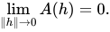
ノルムが微分可能であるためには0 {\displaystyle 0} リム ‖ h ‖ → 0 A ( h ) = 0. {\displaystyle \lim _{\|h\|\to 0}A(h)=0.}
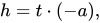
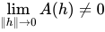
これはどのケースにも当てはまらないことを示す。1 。 {\displaystyle a.} 1 = 0 {\displaystyle a=0} A ( h ) = 1 {\displaystyle A(h)=1} h 、 {\displaystyle h,} 1 ≠ 0. {\displaystyle a\neq 0.} h {\displaystyle h} − 1 {\displaystyle -a} h = t ⋅ ( − 1 ) 、 {\displaystyle h=t\cdot (-a),} t → 0 + {\displaystyle t\to 0^{+}} A ( h ) = | 1 + ‖ 1 ‖ | > 1 > 0 、 {\displaystyle A(h)=|1+\|a\||>1>0,} リム ‖ h ‖ → 0 A ( h ) ≠ 0 {\displaystyle \lim _{\|h\|\to 0}A(h)\neq 0}
(もし私たちがh {\displaystyle h} 1 {\displaystyle a} | 1 − ‖ 1 ‖ | {\displaystyle |1-\|a\||}
得られた結果は、有限次元における結果と一致する。
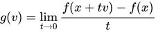
ガトー微分との関係 関数f : U ⊆ V → W {\displaystyle f:U\subseteq V\to W} ガトーと呼ばれ、微分 x ∈ U {\displaystyle x\in U} f {\displaystyle f} x 。 {\displaystyle x.} g : V → W {\displaystyle g:V\to W} g ( v ) = lim t → 0 f ( x + t v ) − f ( x ) t {\displaystyle g(v)=\lim _{t\to 0}{\frac {f(x+tv)-f(x)}{t}}} v ∈ V , {\displaystyle v\in V,} t {\displaystyle t} V {\displaystyle V} t {\displaystyle t} real ).[ 4]
If f {\displaystyle f} x , {\displaystyle x,} g {\displaystyle g} A = D f ( x ) . {\displaystyle A=Df(x).}
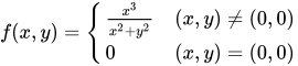
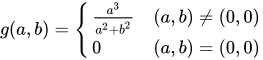
However, not every Gateaux differentiable function is Fréchet differentiable. This is analogous to the fact that the existence of all directional derivatives at a point does not guarantee total differentiability (or even continuity) at that point. For example, the real-valued function f {\displaystyle f} f ( x , y ) = { x 3 x 2 + y 2 ( x , y ) ≠ ( 0 , 0 ) 0 ( x , y ) = ( 0 , 0 ) {\displaystyle f(x,y)={\begin{cases}{\frac {x^{3}}{x^{2}+y^{2}}}&(x,y)\neq (0,0)\\0&(x,y)=(0,0)\end{cases}}} ( 0 , 0 ) {\displaystyle (0,0)} g ( a , b ) = { a 3 a 2 + b 2 ( a , b ) ≠ ( 0 , 0 ) 0 ( a , b ) = ( 0 , 0 ) {\displaystyle g(a,b)={\begin{cases}{\frac {a^{3}}{a^{2}+b^{2}}}&(a,b)\neq (0,0)\\0&(a,b)=(0,0)\end{cases}}}
The function g {\displaystyle g}
More generally, any function of the form f ( x , y ) = g ( r ) h ( ϕ ) , {\displaystyle f(x,y)=g(r)h(\phi ),} r {\displaystyle r} ϕ {\displaystyle \phi } polar coordinates of ( x , y ) , {\displaystyle (x,y),} ( 0 , 0 ) {\displaystyle (0,0)} g {\displaystyle g} 0 {\displaystyle 0} h ( ϕ + π ) = − h ( ϕ ) , {\displaystyle h(\phi +\pi )=-h(\phi ),} h {\displaystyle h} sinusoidal .
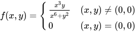
In another situation, the function f {\displaystyle f} f ( x , y ) = { x 3 y x 6 + y 2 ( x , y ) ≠ ( 0 , 0 ) 0 ( x , y ) = ( 0 , 0 ) {\displaystyle f(x,y)={\begin{cases}{\frac {x^{3}y}{x^{6}+y^{2}}}&(x,y)\neq (0,0)\\0&(x,y)=(0,0)\end{cases}}} ( 0 , 0 ) , {\displaystyle (0,0),} g ( a , b ) = 0 {\displaystyle g(a,b)=0} ( a , b ) , {\displaystyle (a,b),} is a linear operator. However, f {\displaystyle f} ( 0 , 0 ) {\displaystyle (0,0)} ( t , t 3 ) {\displaystyle \left(t,t^{3}\right)} f {\displaystyle f}
A more subtle example is f ( x , y ) = { x 2 y x 4 + y 2 x 2 + y 2 ( x , y ) ≠ ( 0 , 0 ) 0 ( x , y ) = ( 0 , 0 ) {\displaystyle f(x,y)={\begin{cases}{\frac {x^{2}y}{x^{4}+y^{2}}}{\sqrt {x^{2}+y^{2}}}&(x,y)\neq (0,0)\\0&(x,y)=(0,0)\end{cases}}} ( 0 , 0 ) , {\displaystyle (0,0),} g ( a , b ) = 0 {\displaystyle g(a,b)=0} f {\displaystyle f} A = 0 {\displaystyle A=0} lim ‖ h ‖ 2 → 0 | f ( ( 0 , 0 ) + h ) − f ( 0 , 0 ) − A h | ‖ h ‖ 2 = lim h = ( x , y ) → ( 0 , 0 ) | x 2 y x 4 + y 2 | {\displaystyle \lim _{\|h\|_{2}\to 0}{\frac {|f((0,0)+h)-f(0,0)-Ah|}{\|h\|_{2}}}=\lim _{h=(x,y)\to (0,0)}\left|{\frac {x^{2}y}{x^{4}+y^{2}}}\right|} ( t , t 2 ) {\displaystyle \left(t,t^{2}\right)}
These cases can occur because the definition of the Gateaux derivative only requires that the difference quotients converge along each direction individually, without making requirements about the rates of convergence for different directions. Thus, for a given ε, although for each direction the difference quotient is within ε of its limit in some neighborhood of the given point, these neighborhoods may be different for different directions, and there may be a sequence of directions for which these neighborhoods become arbitrarily small. If a sequence of points is chosen along these directions, the quotient in the definition of the Fréchet derivative, which considers all directions at once, may not converge. Thus, in order for a linear Gateaux derivative to imply the existence of the Fréchet derivative, the difference quotients have to converge uniformly for all directions.
The following example only works in infinite dimensions. Let X {\displaystyle X} φ {\displaystyle \varphi } 汎 関数X {\displaystyle X} 不連続 ですx = 0 {\displaystyle x=0} 不連続な線形汎関数 )。 f ( x ) = ‖ x ‖ φ ( x ) 。 {\displaystyle f(x)=\|x\|\varphi (x).}
それからf ( x ) {\displaystyle f(x)} x = 0 {\displaystyle x=0} 0. {\displaystyle 0.} f ( x ) {\displaystyle f(x)} リム x → 0 φ ( x ) {\displaystyle \lim _{x\to 0}\varphi (x)}
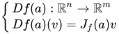
高階微分 もしf : U → W {\displaystyle f:U\to W} U {\displaystyle U} V 、 {\displaystyle V,} D f : U → L ( V 、 W ) {\displaystyle Df:U\to L(V,W)} U {\displaystyle U} L ( V 、 W ) {\displaystyle L(V,W)} V {\displaystyle V} W 。 {\displaystyle W.} 2 階導関数も存在する可能性がある。 f 、 {\displaystyle f,} D 2 f : U → L ( V 、 L ( V 、 W ) ) 。 {\displaystyle D^{2}f:U\to L(V,L(V,W)).}
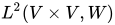
2階微分を扱いやすくするために、右辺の空間はバナッハ空間と同一視される。L 2 ( V × V 、 W ) {\displaystyle L^{2}(V\times V,W)} 双線形写像 からV {\displaystyle V} W 。 {\displaystyle W.} φ {\displaystyle \varphi } L ( V 、 L ( V 、 W ) ) {\displaystyle L(V,L(V,W))} ψ {\displaystyle \psi } L 2 ( V × V 、 W ) {\displaystyle L^{2}(V\times V,W)} x 、 y ∈ V 、 {\displaystyle x,y\in V,} φ ( x ) ( y ) = ψ ( x 、 y ) 。 {\displaystyle \varphi (x)(y)=\psi (x,y).}
(直感的に言えば、関数φ {\displaystyle \varphi } x {\displaystyle x} φ ( x ) {\displaystyle \varphi (x)} y {\displaystyle y} ψ {\displaystyle \psi } x {\displaystyle x} y {\displaystyle y}
区別することができる D 2 f : U → L 2 ( V × V 、 W ) {\displaystyle D^{2}f:U\to L^{2}(V\times V,W)} 再び、 3階微分 を求めると、各点で3次線形写像 となり、以下同様となる。n {\displaystyle n} D n f : U → L n ( V × V × ⋯ × V 、 W ) 、 {\displaystyle D^{n}f:U\to L^{n}(V\times V\times \cdots \times V,W),} 連続多重線形写像 のバナッハ空間で値を取るn {\displaystyle n} V {\displaystyle V} W 。 {\displaystyle W.} f {\displaystyle f} n + 1 {\displaystyle n+1} U {\displaystyle U} n {\displaystyle n} U {\displaystyle U} x ∈ U {\displaystyle x\in U} A {\displaystyle A} n + 1 {\displaystyle n+1} リム h n + 1 → 0 ‖ D n f ( x + h n + 1 ) ( h 1 、 h 2 、 … 、 h n ) − D n f ( x ) ( h 1 、 h 2 、 … 、 h n ) − A ( h 1 、 h 2 、 … 、 h n 、 h n + 1 ) ‖ ‖ h n + 1 ‖ = 0 {\displaystyle \lim _{h_{n+1}\to 0}{\frac {\left\|D^{n}f\left(x+h_{n+1}\right)(h_{1},h_{2},\ldots ,h_{n})-D^{n}f(x)(h_{1},h_{2},\ldots ,h_{n})-A\left(h_{1},h_{2},\ldots ,h_{n},h_{n+1}\right)\right\|}{\left\|h_{n+1}\right\|}}=0} 均一に 存在 するh 1 、 h 2 、 … 、 h n {\displaystyle h_{1},h_{2},\ldots ,h_{n}} V 。 {\displaystyle V.} A {\displaystyle A} ( n + 1 ) {\displaystyle (n+1)} f {\displaystyle f} x 。 {\displaystyle x.}
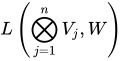
さらに、テンソル積 の定義により、空間の要素を特定することができる。L n ( V × V × ⋯ × V 、 W ) {\displaystyle L^{n}\left(V\times V\times \cdots \times V,W\right)} L ( ⨂ j = 1 n V j 、 W ) {\displaystyle L\left(\bigotimes _{j=1}^{n}V_{j},W\right)} f ( x 1 、 x 2 、 … 、 x n ) = f ( x 1 ⊗ x 2 ⊗ ⋯ ⊗ x n ) 、 {\displaystyle f\left(x_{1},x_{2},\ldots ,x_{n}\right)=f\left(x_{1}\otimes x_{2}\otimes \cdots \otimes x_{n}\right),}
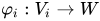
このセクションでは、次の形式の関数に対して定義される偏微分 の概念を拡張します。f : R n → R 、 {\displaystyle f:\mathbb {R} ^{n}\to \mathbb {R} ,} バナッハ空間で ある関数に対して、V 1 、 … 、 V n {\displaystyle V_{1},\ldots ,V_{n}} W {\displaystyle W} f : ∏ 私 = 1 n V 私 → W {\textstyle f:\prod _{i=1}^{n}V_{i}\to W} 1 = ( 1 1 、 … 、 1 n ) ∈ ∏ 私 = 1 n V 私 。 {\textstyle a=\left(a_{1},\ldots ,a_{n}\right)\in \prod _{i=1}^{n}V_{i}.} f {\displaystyle f} 1 {\displaystyle a} φ 私 : V 私 → W {\displaystyle \varphi _{i}:V_{i}\to W}
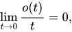
φ 私 ( x ) = f ( 1 1 、 … 、 1 私 − 1 、 x 、 1 私 + 1 、 … 1 n ) {\displaystyle \varphi _{i}(x)=f(a_{1},\ldots ,a_{i-1},x,a_{i+1},\ldots a_{n})} 1 私 {\displaystyle a_{i}} ∂ 私 f ( 1 ) := D φ 私 ( 1 私 ) 、 {\displaystyle \partial _{i}f(a):=D\varphi _{i}(a_{i}),} ∂ 私 f ( 1 ) {\displaystyle \partial _{i}f(a)} f {\displaystyle f} 1 。 {\displaystyle a.} ∂ 私 f ( 1 ) {\displaystyle \partial _{i}f(a)} V 私 {\displaystyle V_{i}} W 。 {\displaystyle W.} f {\displaystyle f} 1 、 {\displaystyle a,} ∂ 私 f ( 1 ) {\displaystyle \partial _{i}f(a)} f {\displaystyle f} 1 j {\displaystyle a_{j}} j ≠ 私 、 {\displaystyle j\neq i,} f ( 1 1 、 … 、 1 私 + h 、 … 1 n ) − f ( 1 1 、 … 、 1 n ) = ∂ 私 f ( 1 ) ( h ) + o ( h ) 。 {\displaystyle f(a_{1},\ldots ,a_{i}+h,\ldots a_{n})-f(a_{1},\ldots ,a_{n})=\partial _{i}f(a)(h)+o(h).}
注記 ↑ イリイン、VA; ポズニャク、EG (1982).数学解析の基礎 . 第 1巻. イレーネ・アレクサノワによるロシア語からの翻訳. ミール出版社、モスクワ. pp. 497–498 . ISBN 978-93-859-2386-9 。 ↑ ブロンシュタイン、イリヤ N.;セメンジャエフ、コンスタンチン A.ゲルハルト・ムジオル。ミューリッグ、ハイナー (2007)。 数学ハンドブック (第 5 版)。シュプリンガー・ベルリン、ハイデルベルク。 p. 394.ISBN 978-3-540-72121-5 。↑ ルディン、ウォルター (1976). 数学解析の原理 (第 3 版). マグロウヒル社、p. 239. ISBN 0-07-054235-X 。↑ 定義には、結果として得られるマップを含めるのが一般的ですg {\displaystyle g} は連続線形演算子 でなければなりません。ここでは、可能な限り幅広い種類の病理を調査できるように、この慣例を採用しません。
外部リンク BA Frigyik、S. Srivastava、MR Gupta、「関数誘導体入門」 、UWEE 技術レポート 2008-0001。 http://www.probability.netこのウェブページは主に基本的な確率論と測度論に関するものですが、バナッハ空間におけるフレシェ微分に関する優れた章(ヤコビ公式に関する章)もあります。すべての結果は証明付きで示されています。


























![{\displaystyle {\begin{aligned}{\frac {|\|x+h\|-\|x\|-Dh|}{\|h\|}}&={\frac {|\|x\|\|x+h\|-\langle x,x\rangle -\langle x,h\rangle |}{\|x\|\|h\|}}\\[8pt]&={\frac {|\|x\|\|x+h\|-\langle x,x+h\rangle |}{\|x\|\|h\|}}\\[8pt]&={\frac {|\langle x,x\rangle \langle x+h,x+h\rangle -\langle x,x+h\rangle ^{2}|}{\|x\|\|h\|(|\|x\|\|x+h\|+\langle x,x+h\rangle |)}}\\[8pt]&={\frac {\langle x,x\rangle \langle h,h\rangle -\langle x,h\rangle ^{2}}{\|x\|\|h\|(|\|x\|\|x+h\|+\langle x,x+h\rangle |)}}\\&{}\end{aligned}}}](https://wikimedia.org/api/rest_v1/media/math/render/svg/c35a1592e1c1d1b3306ed970cea8d153de659227)
![{\displaystyle {\begin{aligned}\lim _{\|h\|\to 0}{\frac {|\|x+h\|-\|x\|-Dh|}{\|h\|}}&=\lim _{\|h\|\to 0}{\frac {\langle x,x\rangle \langle h,h\rangle -\langle x,h\rangle ^{2}}{\|x\|\|h\|(|\|x\|\|x+h\|+\langle x,x+h\rangle |)}}\\[8pt]&={\frac {1}{2\|x\|^{3}}}\lim _{\|h\|\to 0}{\frac {\langle x,x\rangle \langle h,h\rangle -\langle x,h\rangle ^{2}}{\|h\|}}\\[8pt]&={\frac {1}{2\|x\|^{3}}}\lim _{\|h\|\to 0}\left(\langle x,x\rangle \|h\|-\langle x,h\rangle \left\langle x,{\frac {h}{\|h\|}}\right\rangle \right)\\[8pt]&={\frac {1}{2\|x\|^{3}}}\left(\lim _{\|h\|\to 0}\langle x,x\rangle \|h\|-\lim _{h\to 0}\langle x,h\rangle \left\langle x,{\frac {h}{\|h\|}}\right\rangle \right)\\[8pt]&={\frac {1}{2\|x\|^{3}}}\left(0-\lim _{\|h\|\to 0}\langle x,h\rangle \left\langle x,{\frac {h}{\|h\|}}\right\rangle \right)\\[8pt]&=-{\frac {1}{2\|x\|^{3}}}\left(\lim _{\|h\|\to 0}\langle x,h\rangle \left\langle x,{\frac {h}{\|h\|}}\right\rangle \right)\\[8pt]\end{aligned}}}](https://wikimedia.org/api/rest_v1/media/math/render/svg/e330f412e9d74aa04ffdd73fefcf88f0b9a86b1a)