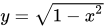
多変数微積分 において、陰関数定理 [ a ] F ( x 、 y ) = 0 {\displaystyle F(x,y)=0} グラフ として指定することもできますf {\displaystyle f} ( x 、 y ) {\displaystyle (x,y)} y = f ( x ) {\displaystyle y=f(x)} 単位円が あり、その点は( x 、 y ) {\displaystyle (x,y)} x 2 + y 2 − 1 = 0 {\displaystyle x^{2}+y^{2}-1=0} y > 0 {\displaystyle y>0} y = 1 − x 2 {\displaystyle y={\sqrt {1-x^{2}}}} F ( x 、 y ) = 0 {\displaystyle F(x,y)=0} y {\displaystyle y} 存在するための解析的条件を与える f {\displaystyle f} f {\displaystyle f}
より一般的には、 m 個の方程式系f i x 1 , ..., x n , y 1 , ..., y m ) = 0、i = 1, ..., m F ( x , y ) = 0 偏微分(各 y i m 個の変数y i は 、その点の近傍 でx j 閉じた形式 で表現できないため、方程式によって暗黙的に定義され、これが定理の名前の由来となっている。 [ 1 ]
言い換えれば、偏導関数に関する緩やかな条件の下では、連立方程式の零点の集合は 局所的に 関数のグラフ となる。
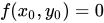
2変数の場合 させてf : R 2 → R {\displaystyle f:\mathbb {R} ^{2}\to \mathbb {R} } 曲線 の陰関数方程式 を定義する連続微分可能な関数であるf ( x 、 y ) = 0 {\displaystyle f(x,y)=0} ( x 0 、 y 0 ) {\displaystyle (x_{0},y_{0})} f ( x 0 、 y 0 ) = 0 {\displaystyle f(x_{0},y_{0})=0}
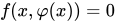
証明。 方程式を微分することにより、 f ( x 、 φ ( x ) ) = 0 {\displaystyle f(x,\varphi (x))=0} ∂ f ∂ x ( x 、 φ ( x ) ) + φ ′ ( x ) ∂ f ∂ y ( x 、 φ ( x ) ) = 0. {\displaystyle {\frac {\partial f}{\partial x}}(x,\varphi (x))+\varphi '(x)\,{\frac {\partial f}{\partial y}}(x,\varphi (x))=0.} φ ′ ( x ) = − ∂ f ∂ x ( x 、 φ ( x ) ) ∂ f ∂ y ( x 、 φ ( x ) ) 。 {\displaystyle \varphi '(x)=-{\frac {{\frac {\partial f}{\partial x}}(x,\varphi (x))}{{\frac {\partial f}{\partial y}}(x,\varphi (x))}}.} 常微分方程式 を与える。 φ {\displaystyle \varphi } 条件 は φ ( x 0 ) = y 0 {\displaystyle \varphi (x_{0})=y_{0}}
以来∂ f ∂ y ( x 0 、 y 0 ) ≠ 0 、 {\textstyle {\frac {\partial f}{\partial y}}(x_{0},y_{0})\neq 0,} ペアノ存在定理が 適用され、(一意ではない可能性もある)解が存在します。その理由を確認するにはφ {\textstyle \varphi } g x ( y ) = f ( x 、 y ) {\textstyle g_{x}(y)=f(x,y)} 単調 であるx 0 、 y 0 {\textstyle x_{0},y_{0}} ∂ f ∂ y ( x 0 、 y 0 ) ≠ 0 {\textstyle {\frac {\partial f}{\partial y}}(x_{0},y_{0})\neq 0} )、したがって単射で ある。φ 、 ϕ {\textstyle \varphi ,\phi } g x ( φ ( x ) ) = g x ( ϕ ( x ) ) = 0 {\textstyle g_{x}(\varphi (x))=g_{x}(\phi (x))=0} φ ( x ) = ϕ ( x ) {\textstyle \varphi (x)=\phi (x)}
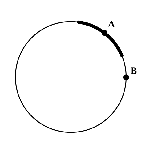
最初の例 陰関数方程式x² + y² – 1 = 0関数 のグラフとして表すことはできません。接線が垂直でない点A の周りでは、太字で示された円弧は x の何らかの関数のグラフですが、点B x の関数は存在しません。これはまさに、この場合の陰関数定理が主張する内容です。関数f ( x , y ) = x 2 + y 2 f ( x , y ) = 1は、レベルセット {( x , y ) | f ( x , y ) = 1} として単位円 を切り取ります。 1 つの変数y = g ( x ) の関数のグラフとして単位円を表す方法はありません。なぜなら、 x ∈ (−1, 1) の各選択に対して、 y には 2 つの選択肢があるからです。± 1 − x 2 {\displaystyle \pm {\sqrt {1-x^{2}}}}
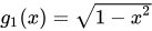
しかし、円の一部を 1変数関数のグラフとして表すことは可能です。g 1 ( x ) = 1 − x 2 {\displaystyle g_{1}(x)={\sqrt {1-x^{2}}}} −1 ≤ x ≤ 1 の場合、 y = g 1 ( x )g 2 ( x ) = − 1 − x 2 {\displaystyle g_{2}(x)=-{\sqrt {1-x^{2}}}} すると、 y = g 2 ( x )
陰関数定理は、いくつかの緩やかな仮定の下では、明示的な式で記述できない状況であっても、g 1 ( x )g 2 ( x )のような関数は常に存在すると述べています。これは、 g 1 ( x )g 2 ( x )が微分可能であることを保証し、 f ( x , y )
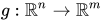
一般的なケース させてf : R n + m → R m {\displaystyle f:\mathbb {R} ^{n+m}\to \mathbb {R} ^{m}} 連続的に微分可能な 関数である。R n + m {\displaystyle \mathbb {R} ^{n+m}} デカルト 積としてR n × R m 、 {\displaystyle \mathbb {R} ^{n}\times \mathbb {R} ^{m},} ( x 、 y ) = ( x 1 、 … 、 x n 、 y 1 、 … y m ) 。 {\displaystyle (\mathbf {x} ,\mathbf {y} )=(x_{1},\ldots ,x_{n},y_{1},\ldots y_{m}).} f {\displaystyle f} g : R n → R m {\displaystyle g:\mathbb {R} ^{n}\to \mathbb {R} ^{m}} ( x 、 g ( x ) ) {\displaystyle ({\textbf {x}},g({\textbf {x}}))} ( x 、 y ) {\displaystyle ({\textbf {x}},{\textbf {y}})} f ( x 、 y ) = 0 {\displaystyle f({\textbf {x}},{\textbf {y}})={\textbf {0}}}
前述のとおり、これは常に可能とは限りません。したがって、ある時点を固定します。( 1 、 b ) = ( 1 1 、 … 、 1 n 、 b 1 、 … 、 b m ) {\displaystyle ({\textbf {a}},{\textbf {b}})=(a_{1},\dots ,a_{n},b_{1},\dots ,b_{m})} f ( 1 、 b ) = 0 {\displaystyle f({\textbf {a}},{\textbf {b}})={\textbf {0}}} g {\displaystyle g} ( 1 、 b ) {\displaystyle ({\textbf {a}},{\textbf {b}})} オープンセットを求めている。 U ⊂ R n {\displaystyle U\subset \mathbb {R} ^{n}} 1 {\displaystyle {\textbf {a}}} V ⊂ R m {\displaystyle V\subset \mathbb {R} ^{m}} b {\displaystyle {\textbf {b}}} g : U → V {\displaystyle g:U\to V} g {\displaystyle g} f = 0 {\displaystyle f={\textbf {0}}} U × V {\displaystyle U\times V} U × V {\displaystyle U\times V}
{ ( x 、 g ( x ) ) ∣ x ∈ U } = { ( x 、 y ) ∈ U × V ∣ f ( x 、 y ) = 0 } 。 {\displaystyle \{(\mathbf {x} ,g(\mathbf {x} ))\mid \mathbf {x} \in U\}=\{(\mathbf {x} ,\mathbf {y} )\in U\times V\mid f(\mathbf {x} ,\mathbf {y} )=\mathbf {0} \}.}
陰関数定理を述べるには、ヤコビ行列 が必要です。f {\displaystyle f} 偏微分 行列である。f {\displaystyle f} ( 1 1 、 … 、 1 n 、 b 1 、 … 、 b m ) {\displaystyle (a_{1},\dots ,a_{n},b_{1},\dots ,b_{m})} ( 1 、 b ) {\displaystyle ({\textbf {a}},{\textbf {b}})}
( D f ) ( 1 、 b ) = [ ∂ f 1 ∂ x 1 ( 1 、 b ) ⋯ ∂ f 1 ∂ x n ( 1 、 b ) ∂ f 1 ∂ y 1 ( 1 、 b ) ⋯ ∂ f 1 ∂ y m ( 1 、 b ) ⋮ ⋱ ⋮ ⋮ ⋱ ⋮ ∂ f m ∂ x 1 ( 1 、 b ) ⋯ ∂ f m ∂ x n ( 1 、 b ) ∂ f m ∂ y 1 ( 1 、 b ) ⋯ ∂ f m ∂ y m ( 1 、 b ) ] = [ X Y ] {\displaystyle (Df)(\mathbf {a} ,\mathbf {b} )=\left[{\begin{array}{ccc|ccc}{\frac {\partial f_{1}}{\partial x_{1}}}(\mathbf {a} ,\mathbf {b} )&\cdots &{\frac {\partial f_{1}}{\partial x_{n}}}(\mathbf {a} ,\mathbf {b} )&{\frac {\partial f_{1}}{\partial y_{1}}}(\mathbf {a} ,\mathbf {b} )&\cdots &{\frac {\partial f_{1}}{\partial y_{m}}}(\mathbf {a} ,\mathbf {b} )\\\vdots &\ddots &\vdots &\vdots &\ddots &\vdots \\{\frac {\partial f_{m}}{\partial x_{1}}}(\mathbf {a} ,\mathbf {b} )&\cdots &{\frac {\partial f_{m}}{\partial x_{n}}}(\mathbf {a} ,\mathbf {b} )&{\frac {\partial f_{m}}{\partial y_{1}}}(\mathbf {a} ,\mathbf {b} )&\cdots &{\frac {\partial f_{m}}{\partial y_{m}}}(\mathbf {a} ,\mathbf {b} )\end{array}}\right]=\left[{\begin{array}{c|c}X&Y\end{array}}\right]}
どこX {\displaystyle X} x 私 {\displaystyle x_{i}} Y {\displaystyle Y} y j {\displaystyle y_{j}} Y {\displaystyle Y} U {\displaystyle U} V {\displaystyle V} g {\displaystyle g}
定理の記述 させてf : R n + m → R m {\displaystyle f:\mathbb {R} ^{n+m}\to \mathbb {R} ^{m}} 連続微分可能な関数 とし、R n + m {\displaystyle \mathbb {R} ^{n+m}} ( x 、 y ) {\displaystyle ({\textbf {x}},{\textbf {y}})} ( 1 、 b ) = ( 1 1 、 … 、 1 n 、 b 1 、 … 、 b m ) {\displaystyle ({\textbf {a}},{\textbf {b}})=(a_{1},\dots ,a_{n},b_{1},\dots ,b_{m})} f ( 1 、 b ) = 0 {\displaystyle f({\textbf {a}},{\textbf {b}})=\mathbf {0} } 0 ∈ R m {\displaystyle \mathbf {0} \in \mathbb {R} ^{m}} ヤコビ行列 (これは前のセクションで示したヤコビ行列の右側のパネルです)の場合: J f 、 y ( 1 、 b ) = [ ∂ f 私 ∂ y j ( 1 、 b ) ] {\displaystyle J_{f,\mathbf {y} }(\mathbf {a} ,\mathbf {b} )=\left[{\frac {\partial f_{i}}{\partial y_{j}}}(\mathbf {a} ,\mathbf {b} )\right]} 可逆で あれば、開集合が存在する。U ⊂ R n {\displaystyle U\subset \mathbb {R} ^{n}} 1 {\displaystyle {\textbf {a}}} g : U → R m {\displaystyle g:U\to \mathbb {R} ^{m}} g ( 1 ) = b {\displaystyle g(\mathbf {a} )=\mathbf {b} } f ( x 、 g ( x ) ) = 0 すべての人々のために x ∈ U {\displaystyle f(\mathbf {x} ,g(\mathbf {x} ))=\mathbf {0} ~{\text{for all}}~\mathbf {x} \in U} g {\displaystyle g} J f 、 x ( 1 、 b ) = [ ∂ f 私 ∂ x j ( 1 、 b ) ] 、 {\displaystyle J_{f,\mathbf {x} }(\mathbf {a} ,\mathbf {b} )=\left[{\frac {\partial f_{i}}{\partial x_{j}}}(\mathbf {a} ,\mathbf {b} )\right],} g {\displaystyle g} U {\displaystyle U} は行列積 によって与えられる:[ 3 ] [ ∂ g 私 ∂ x j ( x ) ] m × n = − [ J f 、 y ( x 、 g ( x ) ) ] m × m − 1 [ J f 、 x ( x 、 g ( x ) ) ] m × n {\displaystyle \left[{\frac {\partial g_{i}}{\partial x_{j}}}(\mathbf {x} )\right]_{m\times n}=-\left[J_{f,\mathbf {y} }(\mathbf {x} ,g(\mathbf {x} ))\right]_{m\times m}^{-1}\,\left[J_{f,\mathbf {x} }(\mathbf {x} ,g(\mathbf {x} ))\right]_{m\times n}}
証明は逆関数定理に関する 記事に記載されています。ここでは、2次元の場合について詳しく説明します。
アプリケーション:座標変更 m 次元空間があり、それが一連の座標によってパラメータ化されていると仮定します。( x 1 、 … 、 x m ) {\displaystyle (x_{1},\ldots ,x_{m})} ( x 1 ′ 、 … 、 x m ′ ) {\displaystyle (x'_{1},\ldots ,x'_{m})} h 1 … h m {\displaystyle h_{1}\ldots h_{m}} ( x 1 ′ 、 … 、 x m ′ ) {\displaystyle (x'_{1},\ldots ,x'_{m})} ( x 1 、 … 、 x m ) {\displaystyle (x_{1},\ldots ,x_{m})} x 1 ′ = h 1 ( x 1 、 … 、 x m ) 、 … 、 x m ′ = h m ( x 1 、 … 、 x m ) {\displaystyle x'_{1}=h_{1}(x_{1},\ldots ,x_{m}),\ldots ,x'_{m}=h_{m}(x_{1},\ldots ,x_{m})} ( x 1 ′ 、 … 、 x m ′ ) {\displaystyle (x'_{1},\ldots ,x'_{m})} ( x 1 、 … 、 x m ) {\displaystyle (x_{1},\ldots ,x_{m})} ( x 1 ′ 、 … 、 x m ′ 、 x 1 、 … 、 x m ) {\displaystyle (x'_{1},\ldots ,x'_{m},x_{1},\ldots ,x_{m})} f = 0 で関係付けられ、f ( x 1 ′ 、 … 、 x m ′ 、 x 1 、 … 、 x m ) = ( h 1 ( x 1 、 … 、 x m ) − x 1 ′ 、 … 、 h m ( x 1 、 … 、 x m ) − x m ′ ) 。 {\displaystyle f(x'_{1},\ldots ,x'_{m},x_{1},\ldots ,x_{m})=(h_{1}(x_{1},\ldots ,x_{m})-x'_{1},\ldots ,h_{m}(x_{1},\ldots ,x_{m})-x'_{m}).} a , b )におけるf のヤコビ行列は、1 = ( x 1 ′ 、 … 、 x m ′ ) 、 b = ( x 1 、 … 、 x m ) {\displaystyle a=(x'_{1},\ldots ,x'_{m}),b=(x_{1},\ldots ,x_{m})} ( D f ) ( 1 、 b ) = [ − 1 ⋯ 0 ⋮ ⋱ ⋮ 0 ⋯ − 1 | ∂ h 1 ∂ x 1 ( b ) ⋯ ∂ h 1 ∂ x m ( b ) ⋮ ⋱ ⋮ ∂ h m ∂ x 1 ( b ) ⋯ ∂ h m ∂ x m ( b ) ] = [ − 私 m | J ] 。 {\displaystyle (Df)(a,b)=\left[{\begin{matrix}-1&\cdots &0\\\vdots &\ddots &\vdots \\0&\cdots &-1\end{matrix}}\left|{\begin{matrix}{\frac {\partial h_{1}}{\partial x_{1}}}(b)&\cdots &{\frac {\partial h_{1}}{\partial x_{m}}}(b)\\\vdots &\ddots &\vdots \\{\frac {\partial h_{m}}{\partial x_{1}}}(b)&\cdots &{\frac {\partial h_{m}}{\partial x_{m}}}(b)\\\end{matrix}}\right.\right]=[-I_{m}|J].} m は m × m の 単位行列 を表し、J は( a , b )で評価された偏導関数のm × m a に依存しません。)陰関数定理は、局所的に表現できることを示しています。( x 1 、 … 、 x m ) {\displaystyle (x_{1},\ldots ,x_{m})} ( x 1 ′ 、 … 、 x m ′ ) {\displaystyle (x'_{1},\ldots ,x'_{m})} J が可逆である場合。J が可逆であるという要求はdet J ≠ 0 と同等であるため、ヤコビ行列 J の行列式がゼロでない場合、プライム付き座標からプライムなし座標に戻ることができることがわかります。この記述は逆関数定理 としても知られています。
例:極座標 上記の簡単な応用として、極座標 ( R , θ ) でパラメータ化された平面を考えます。関数x ( R , θ ) = R cos( θ ) およびy ( R , θ ) = R sin( θ )を定義することで、新しい座標系 ( デカルト座標) に移行できます。これにより、任意の点 ( R , θ )に対して、対応するデカルト座標 ( x , y ) を求めることができます。デカルト座標から極座標に戻ることができるのはどのような場合でしょうか。前の例から、 det J ≠ 0 で 十分です。J = [ ∂ x ( R 、 θ ) ∂ R ∂ x ( R 、 θ ) ∂ θ ∂ y ( R 、 θ ) ∂ R ∂ y ( R 、 θ ) ∂ θ ] = [ コス θ − R 罪 θ 罪 θ R コス θ ] 。 {\displaystyle J={\begin{bmatrix}{\frac {\partial x(R,\theta )}{\partial R}}&{\frac {\partial x(R,\theta )}{\partial \theta }}\\{\frac {\partial y(R,\theta )}{\partial R}}&{\frac {\partial y(R,\theta )}{\partial \theta }}\\\end{bmatrix}}={\begin{bmatrix}\cos \theta &-R\sin \theta \\\sin \theta &R\cos \theta \end{bmatrix}}.} det J = R なので、 R ≠ 0R = 0= 0 の
一般化
バナッハ宇宙版 バナッハ空間 における逆関数定理 に基づき、陰関数定理をバナッハ空間値写像に拡張することが可能です。[ 5 ] [ 6 ]
X 、Y 、Zを バナッハ空間 とする。写像f : X × Y → Z フレシェ微分可能 であるとする。( x 0 、 y 0 ) ∈ X × Y {\displaystyle (x_{0},y_{0})\in X\times Y} f ( x 0 、 y 0 ) = 0 {\displaystyle f(x_{0},y_{0})=0} y ↦ D f ( x 0 、 y 0 ) ( 0 、 y ) {\displaystyle y\mapsto Df(x_{0},y_{0})(0,y)} Yから Z へのバナッハ空間同型写像が存在するならば、x 0 の近傍U とy 0 の近傍Vが 存在 し、すべてのxに対して f ( x , g ( x )) = 0 かつf ( x , y ) = 0となるのはy = g ( x )の場合のみであるようなフレシェ微分可能な関数g : U → V が存在する。 ( x 、 y ) ∈ U × V {\displaystyle (x,y)\in U\times V}
参考文献 ↑ Chiang, Alpha C. (1984). Fundamental Methods of Mathematical Economics (3rd ed.). McGraw-Hill. pp. 204–206 . ISBN 0-07-010813-7 。↑ クランツ、スティーブン;パークス、ハロルド(2003)。 陰関数定理 。モダン・バークハウザー・クラシックス。バークハウザー 。ISBN 0-8176-4285-4 。↑ de Oliveira, Oswaldo (2013). "The Implicit and Inverse Function Theorems: Easy Proofs". Real Anal. Exchange . 39 (1): 214– 216. arXiv : 1212.2066 . doi : 10.14321/realanalexch.39.1.0207 . S2CID 118792515 . ↑ フリッチェ、K.; グラウアート、H. (2002)。 正則関数から複素多様体まで 。スプリンガー。 p. 34.ISBN 9780387953953 。↑ ラング、セルジュ (1999). 微分幾何学の基礎 . 大学院数学テキスト. ニューヨーク: スプリンガー. pp. 15 –21. ISBN 0-387-98593-X 。↑ エドワーズ、チャールズ・ヘンリー (1994) [1973]. 多変数高等微積分 . ミネオラ、ニューヨーク: ドーバー出版. pp. 417–418 . ISBN 0-486-68336-2 。↑ クドリャフツェフ、レフ・ドミトリエヴィチ (2001) [1994]、 「陰関数」 、 数学百科事典 、EMS Press ↑ Jittorntrum, K. (1978). "An Implicit Function Theorem". Journal of Optimization Theory and Applications . 25 (4): 575–577 . doi : 10.1007/BF00933522 . S2CID 121647783 . ↑ 熊谷 茂( 1980)「陰関数定理:コメント」 最適化理論と応用ジャーナル 31 ( 2 ) : 285–288。doi : 10.1007/ BF00934117。S2CID 119867925 。 ↑ 曹操、建国。ゲー・ジャン(2011)。 「3多様体に対するペレルマンの崩壊定理の簡単な証明」。 J.Geom.アナル 。 21 (4 ) : 807–869.arXiv : 1003.2215 。 土井 : 10.1007/s12220-010-9169-5 。 S2CID 514106 。 11 Generalized Implicit Function Theorem Journal Of Indonesian Mathematical Society DOI:10.22.342 v3211.1551 License CCBY-NC-ND-4.0 Discusses Implicit function Theorem for X a topological space , Y Banach Space, Z a Topological Vector space
Further reading Allendoerfer, Carl B. (1974). "Theorems about Differentiable Functions". Calculus of Several Variables and Differentiable Manifolds . New York: Macmillan. pp. 54– 88. ISBN 0-02-301840-2 .Binmore, K. G. (1983). "Implicit Functions". Calculus . New York: Cambridge University Press. pp. 198– 211. ISBN 0-521-28952-1 .Loomis, Lynn H. ; Sternberg, Shlomo (1990). Advanced Calculus ed.). Boston: Jones and Bartlett. pp. 164–171. ISBN 0-86720-122-3 .Protter, Murray H. ; Morrey, Charles B. Jr. (1985). "Implicit Function Theorems. Jacobians". Intermediate Calculus (2nd ed.). New York: Springer. pp. 390– 420. ISBN 0-387-96058-9 .






















![{\displaystyle (Df)(\mathbf {a} ,\mathbf {b} )=\left[{\begin{array}{ccc|ccc}{\frac {\partial f_{1}}{\partial x_{1}}}(\mathbf {a} ,\mathbf {b} )&\cdots &{\frac {\partial f_{1}}{\partial x_{n}}}(\mathbf {a} ,\mathbf {b} )&{\frac {\partial f_{1}}{\partial y_{1}}}(\mathbf {a} ,\mathbf {b} )&\cdots &{\frac {\partial f_{1}}{\partial y_{m}}}(\mathbf {a} ,\mathbf {b} )\\\vdots &\ddots &\vdots &\vdots &\ddots &\vdots \\{\frac {\partial f_{m}}{\partial x_{1}}}(\mathbf {a} ,\mathbf {b} )&\cdots &{\frac {\partial f_{m}}{\partial x_{n}}}(\mathbf {a} ,\mathbf {b} )&{\frac {\partial f_{m}}{\partial y_{1}}}(\mathbf {a} ,\mathbf {b} )&\cdots &{\frac {\partial f_{m}}{\partial y_{m}}}(\mathbf {a} ,\mathbf {b} )\end{array}}\right]=\left[{\begin{array}{c|c}X&Y\end{array}}\right]}](https://wikimedia.org/api/rest_v1/media/math/render/svg/4ed6c59b149f9092cf52e03fdb1d36423622f356)


![{\displaystyle J_{f,\mathbf {y} }(\mathbf {a} ,\mathbf {b} )=\left[{\frac {\partial f_{i}}{\partial y_{j}}}(\mathbf {a} ,\mathbf {b} )\right]}](https://wikimedia.org/api/rest_v1/media/math/render/svg/23fa28aac64bb9a2ec05d198291b291cfc040c4e)



![{\displaystyle J_{f,\mathbf {x} }(\mathbf {a} ,\mathbf {b} )=\left[{\frac {\partial f_{i}}{\partial x_{j}}}(\mathbf {a} ,\mathbf {b} )\right],}](https://wikimedia.org/api/rest_v1/media/math/render/svg/5dca6d13ba18d76dd877c869803e9575ca7f91b3)
![${\displaystyle \left[{\frac {\partial g_{i}}{\partial x_{j}}}(\mathbf {x} )\right]_{m\times n}=-\left[J_{f,\mathbf {y} }(\mathbf {x} ,g(\mathbf {x} ))\right]_{m\times m}^{-1}\,\left[J_{f,\mathbf {x} }(\mathbf {x} ,g(\mathbf {x} ))\right]_{m\times n}}$](https://wikimedia.org/api/rest_v1/media/math/render/svg/f91c52a4f75b5a475156d03f4e2d12175e5be8bb)












![{\displaystyle (Df)(a,b)=\left[{\begin{matrix}-1&\cdots &0\\\vdots &\ddots &\vdots \\0&\cdots &-1\end{matrix}}\left|{\begin{matrix}{\frac {\partial h_{1}}{\partial x_{1}}}(b)&\cdots &{\frac {\partial h_{1}}{\partial x_{m}}}(b)\\\vdots &\ddots &\vdots \\{\frac {\partial h_{m}}{\partial x_{1}}}(b)&\cdots &{\frac {\partial h_{m}}{\partial x_{m}}}(b)\\\end{matrix}}\right.\right]=[-I_{m}|J].}](https://wikimedia.org/api/rest_v1/media/math/render/svg/1ecb08835787c4ce30095f49de340414e7202bdc)










