
Loading article…
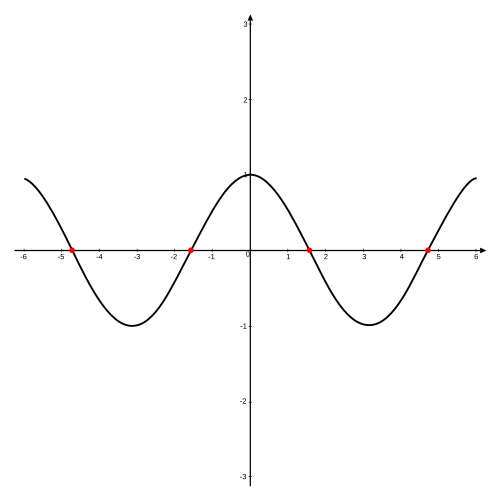
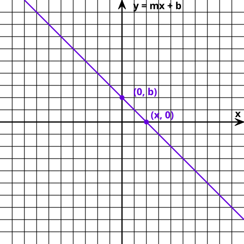
数学において、実数値関数、複素数値関数、または一般的にベクトル値関数の零点(根とも呼ばれる)はメンバーですの領域そのため消える;つまり、関数0 の値に達するまたは同等に、は方程式の解です関数の「ゼロ」とは、出力が0になる入力値のことである。[ 1 ]
多項式の根とは、対応する多項式関数の零点のことである。[ 2 ]代数学の基本定理によれば、零でない多項式は次数以下の根を持ち、複素根(より一般的には、代数的に閉じた拡張における根)を重複度で数えると、根の数と次数は等しくなる。[ 3 ]例えば、多項式次数が2で、次のように定義される。2と3という2つの根(または零点)を持つ。
未知数を含むすべての方程式次のように書き換えることができます
左辺のすべての項をまとめると、このような方程式の解は関数の零点と正確に一致することがわかります。言い換えれば、「関数の零点」とはまさに「関数を0に等しいとおくことによって得られる方程式の解」であり、関数の零点の研究は方程式の解の研究と全く同じである。
Every real polynomial of odd degree has an odd number of real roots (counting multiplicities); likewise, a real polynomial of even degree must have an even number of real roots. Consequently, real odd polynomials must have at least one real root (because the smallest odd whole number is 1), whereas even polynomials may have none. This principle can be proven by reference to the intermediate value theorem: since polynomial functions are continuous, the function value must cross zero, in the process of changing from negative to positive or vice versa (which always happens for odd functions).
The fundamental theorem of algebra states that every polynomial of degree has complex roots, counted with their multiplicities. The non-real roots of polynomials with real coefficients come in conjugate pairs.[1]Vieta's formulas relate the coefficients of a polynomial to sums and products of its roots.
There are many methods for computing accurate approximations of roots of functions, the best being Newton's method, see Root-finding algorithm.
For polynomials, there are specialized algorithms that are more efficient and may provide all roots or all real roots; see Polynomial root-finding and Real-root isolation.
Some polynomial, including all those of degree no greater than 4, can have all their roots expressed algebraically in terms of their coefficients; see Solution in radicals.
In various areas of mathematics, the zero set of a function is the set of all its zeros. More precisely, if is a real-valued function (or, more generally, a function taking values in some additive group), its zero set is , the inverse image of in .
Under the same hypothesis on the codomain of the function, a level set of a function is the zero set of the function for some in the codomain of
The zero set of a linear map is also known as its kernel.
The cozero set of the function is the complement of the zero set of (i.e., the subset of on which is nonzero).
In algebraic geometry, the first definition of an algebraic variety is through zero sets. Specifically, an affine algebraic set is the intersection of the zero sets of several polynomials, in a polynomial ring over a field. In this context, a zero set is sometimes called a zero locus.
In analysis and geometry, any closed subset of is the zero set of a smooth function defined on all of . This extends to any smooth manifold as a corollary of paracompactness.
In differential geometry, zero sets are frequently used to define manifolds. An important special case is the case that is a smooth function from to . If zero is a regular value of , then the zero set of is a smooth manifold of dimension by the regular value theorem.
For example, the unit -sphere in is the zero set of the real-valued function .


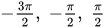
![{\displaystyle \left[-2\pi ,2\pi \right]}](https://wikimedia.org/api/rest_v1/media/math/render/svg/cdc6c1efef56b12d350b9e16f34e39e317d5b51f)






![{\displaystyle k\left[x_{1},\ldots ,x_{n}\right]}](https://wikimedia.org/api/rest_v1/media/math/render/svg/26e790118352b6852ad6a2e132d4c9819b896c45)


