行列の数学演算
数学 において 、クロネッカー積( クロネッカーけっぷ、英: Kronecker product )は、 2つの 行列を 任意の大きさで演算して ブロック行列を生成する 演算 である。これは、 テンソル積 (同じ記号で表記される)をベクトルから行列に特殊化したものであって、標準的な 基底 の選択に関して テンソル積線形写像の行列を与える。クロネッカー積は、全く異なる演算である通常の 行列乗算 とは区別される 。クロネッカー積は、 行列直積 と呼ばれることもある。 [1]
クロネッカー積はドイツの数学者 レオポルト・クロネッカー (1823-1891)にちなんで名付けられたが、彼が最初に定義し使用したという証拠はほとんどない。クロネッカー積は、1858年にこの行列演算を説明した ヨハン・ゲオルク・ツェフス [ドイツ]にちなんで、 ツェフス行列 や ツェフス積 とも呼ばれてきたが、現在ではクロネッカー積という用語が最も広く使われている。 [2] [3]ツェフスではなくクロネッカーに誤って帰属させたのは、 クルト・ヘンゼル によるものである 。 [4]
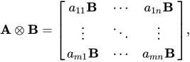
意味 A が m × n 行列で B が p × q 行列の場合 、 クロネッカー積 A⊗B は pm × qn ブロック行列です 。
あ
⊗
B
=
[
1つの
11
B
⋯
1つの
1 ん
B
⋮
⋱
⋮
1つの
メートル 1
B
⋯
1つの
メートル ん
B
]
、
{\displaystyle \mathbf {A} \otimes \mathbf {B} ={\begin{bmatrix}a_{11}\mathbf {B} &\cdots &a_{1n}\mathbf {B} \\\vdots &\ddots &\vdots \\a_{m1}\mathbf {B} &\cdots &a_{mn}\mathbf {B} \end{bmatrix}},}
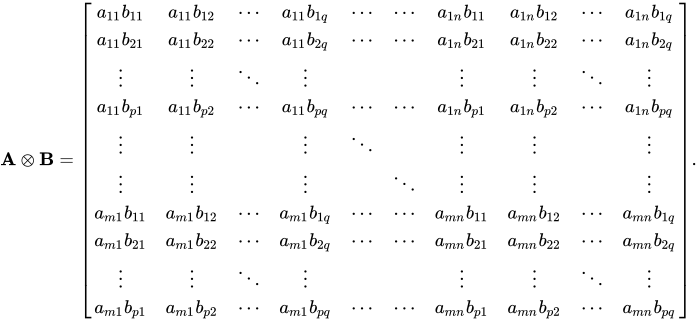
より明確に言えば:
あ
⊗
B
=
[
1つの
11
b
11
1つの
11
b
12
⋯
1つの
11
b
1 q
⋯
⋯
1つの
1 ん
b
11
1つの
1 ん
b
12
⋯
1つの
1 ん
b
1 q
1つの
11
b
21
1つの
11
b
22
⋯
1つの
11
b
2 q
⋯
⋯
1つの
1 ん
b
21
1つの
1 ん
b
22
⋯
1つの
1 ん
b
2 q
⋮
⋮
⋱
⋮
⋮
⋮
⋱
⋮
1つの
11
b
p 1
1つの
11
b
p 2
⋯
1つの
11
b
p q
⋯
⋯
1つの
1 ん
b
p 1
1つの
1 ん
b
p 2
⋯
1つの
1 ん
b
p q
⋮
⋮
⋮
⋱
⋮
⋮
⋮
⋮
⋮
⋮
⋱
⋮
⋮
⋮
1つの
メートル 1
b
11
1つの
メートル 1
b
12
⋯
1つの
メートル 1
b
1 q
⋯
⋯
1つの
メートル ん
b
11
1つの
メートル ん
b
12
⋯
1つの
メートル ん
b
1 q
1つの
メートル 1
b
21
1つの
メートル 1
b
22
⋯
1つの
メートル 1
b
2 q
⋯
⋯
1つの
メートル ん
b
21
1つの
メートル ん
b
22
⋯
1つの
メートル ん
b
2 q
⋮
⋮
⋱
⋮
⋮
⋮
⋱
⋮
1つの
メートル 1
b
p 1
1つの
メートル 1
b
p 2
⋯
1つの
メートル 1
b
p q
⋯
⋯
1つの
メートル ん
b
p 1
1つの
メートル ん
b
p 2
⋯
1つの
メートル ん
b
p q
]
。
{\displaystyle {\mathbf {A} \otimes \mathbf {B} }={\begin{bmatrix}a_{11}b_{11}&a_{11}b_{12}&\cdots &a_{11}b_{1q}&\cdots &\cdots &a_{1n}b_{11}&a_{1n}b_{12}&\cdots &a_{1n}b_{1q}\\a_{11}b_{21}&a_{11}b_{22}&\cdots &a_{11}b_{2q}&\cdots &\cdots &a_{1n}b_{21}&a_{1n}b_{22}&\cdots &a_{1n}b_{2q}\\\vdots &\vdots &\ddots &\vdots &&&\vdots &\vdots &\ddots &\vdots \\a_{11}b_{p1}&a_{11}b_{p2}&\cdots &a_{11}b_{pq}&\cdots &\cdots &a_{1n}b_{p1}&a_{1n}b_{p2}&\cdots &a_{1n}b_{pq}\\\vdots &\vdots &&\vdots &\ddots &&\vdots &\vdots &&\vdots \\\vdots &\vdots &&\vdots &&\ddots &\vdots &\vdots &\vdots \\a_{m1}b_{11}&a_{m1}b_{12}&\cdots &a_{m1}b_{1q}&\cdots &\cdots &a_{mn}b_{11}&a_{mn}b_{12}&\cdots &a_{mn}b_{1q}\\a_{m1}b_{21}&a_{m1}b_{22}&\cdots &a_{m1}b_{2q}&\cdots &\cdots &a_{mn}b_{21}&a_{mn}b_{22}&\cdots &a_{mn}b_{2q}\\\vdots &\vdots &\ddots &\vdots &&&\vdots &\vdots &\ddots &\vdots \\a_{m1}b_{p1}&a_{m1}b_{p2}&\cdots &a_{m1}b_{pq}&\cdots &\cdots &a_{mn}b_{p1}&a_{mn}b_{p2}&\cdots &a_{mn}b_{pq}\end{bmatrix}}.}
および をそれぞれ 整数除算の切り捨て と 剰余 として表し 、 行列要素を0から番号付けすると、次式が得られます。
/
/
{\displaystyle /\!/}
%
{\displaystyle \%}
(
A
⊗
B
)
p
r
+
v
,
q
s
+
w
=
a
r
s
b
v
w
{\displaystyle (A\otimes B)_{pr+v,qs+w}=a_{rs}b_{vw}}
(
A
⊗
B
)
i
,
j
=
a
i
/
/
p
,
j
/
/
q
b
i
%
p
,
j
%
q
.
{\displaystyle (A\otimes B)_{i,j}=a_{i/\!/p,j/\!/q}b_{i\%p,j\%q}.}
通常の1から始まる番号付けでは、
(
A
⊗
B
)
p
(
r
−
1
)
+
v
,
q
(
s
−
1
)
+
w
=
a
r
s
b
v
w
{\displaystyle (A\otimes B)_{p(r-1)+v,q(s-1)+w}=a_{rs}b_{vw}}
(
A
⊗
B
)
i
,
j
=
a
⌈
i
/
p
⌉
,
⌈
j
/
q
⌉
b
(
i
−
1
)
%
p
+
1
,
(
j
−
1
)
%
q
+
1
.
{\displaystyle (A\otimes B)_{i,j}=a_{\lceil i/p\rceil ,\lceil j/q\rceil }b_{(i-1)\%p+1,(j-1)\%q+1}.}
A と B がそれぞれ 線形変換 V 1 → W 1 と V 2 → W 2 を表す 場合 、 2つのマップの テンソル積は A ⊗ B で表され、これは V 1 ⊗ V 2 → W 1 ⊗ W 2 と同じです。
例
[
1
2
3
4
]
⊗
[
0
5
6
7
]
=
[
1
[
0
5
6
7
]
2
[
0
5
6
7
]
3
[
0
5
6
7
]
4
[
0
5
6
7
]
]
=
[
1
×
0
1
×
5
2
×
0
2
×
5
1
×
6
1
×
7
2
×
6
2
×
7
3
×
0
3
×
5
4
×
0
4
×
5
3
×
6
3
×
7
4
×
6
4
×
7
]
=
[
0
5
0
10
6
7
12
14
0
15
0
20
18
21
24
28
]
.
{\displaystyle {\begin{bmatrix}1&2\\3&4\\\end{bmatrix}}\otimes {\begin{bmatrix}0&5\\6&7\\\end{bmatrix}}={\begin{bmatrix}1{\begin{bmatrix}0&5\\6&7\\\end{bmatrix}}&2{\begin{bmatrix}0&5\\6&7\\\end{bmatrix}}\\3{\begin{bmatrix}0&5\\6&7\\\end{bmatrix}}&4{\begin{bmatrix}0&5\\6&7\\\end{bmatrix}}\\\end{bmatrix}}=\left[{\begin{array}{cc|cc}1\times 0&1\times 5&2\times 0&2\times 5\\1\times 6&1\times 7&2\times 6&2\times 7\\\hline 3\times 0&3\times 5&4\times 0&4\times 5\\3\times 6&3\times 7&4\times 6&4\times 7\\\end{array}}\right]=\left[{\begin{array}{cc|cc}0&5&0&10\\6&7&12&14\\\hline 0&15&0&20\\18&21&24&28\end{array}}\right].}
同様に:
[
1
−
4
7
−
2
3
3
]
⊗
[
8
−
9
−
6
5
1
−
3
−
4
7
2
8
−
8
−
3
1
2
−
5
−
1
]
=
[
8
−
9
−
6
5
−
32
36
24
−
20
56
−
63
−
42
35
1
−
3
−
4
7
−
4
12
16
−
28
7
−
21
−
28
49
2
8
−
8
−
3
−
8
−
32
32
12
14
56
−
56
−
21
1
2
−
5
−
1
−
4
−
8
20
4
7
14
−
35
−
7
−
16
18
12
−
10
24
−
27
−
18
15
24
−
27
−
18
15
−
2
6
8
−
14
3
−
9
−
12
21
3
−
9
−
12
21
−
4
−
16
16
6
6
24
−
24
−
9
6
24
−
24
−
9
−
2
−
4
10
2
3
6
−
15
−
3
3
6
−
15
−
3
]
{\displaystyle {\begin{bmatrix}1&-4&7\\-2&3&3\end{bmatrix}}\otimes {\begin{bmatrix}8&-9&-6&5\\1&-3&-4&7\\2&8&-8&-3\\1&2&-5&-1\end{bmatrix}}=\left[{\begin{array}{cccc|cccc|cccc}8&-9&-6&5&-32&36&24&-20&56&-63&-42&35\\1&-3&-4&7&-4&12&16&-28&7&-21&-28&49\\2&8&-8&-3&-8&-32&32&12&14&56&-56&-21\\1&2&-5&-1&-4&-8&20&4&7&14&-35&-7\\\hline -16&18&12&-10&24&-27&-18&15&24&-27&-18&15\\-2&6&8&-14&3&-9&-12&21&3&-9&-12&21\\-4&-16&16&6&6&24&-24&-9&6&24&-24&-9\\-2&-4&10&2&3&6&-15&-3&3&6&-15&-3\end{array}}\right]}
プロパティ
他の行列演算との関係 双線性 と 結合性 :
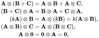
クロネッカー積は テンソル積 の特殊なケースなので、 双線型かつ 結合 的 です。
A
⊗
(
B
+
C
)
=
A
⊗
B
+
A
⊗
C
,
(
B
+
C
)
⊗
A
=
B
⊗
A
+
C
⊗
A
,
(
k
A
)
⊗
B
=
A
⊗
(
k
B
)
=
k
(
A
⊗
B
)
,
(
A
⊗
B
)
⊗
C
=
A
⊗
(
B
⊗
C
)
,
A
⊗
0
=
0
⊗
A
=
0
,
{\displaystyle {\begin{aligned}\mathbf {A} \otimes (\mathbf {B} +\mathbf {C} )&=\mathbf {A} \otimes \mathbf {B} +\mathbf {A} \otimes \mathbf {C} ,\\(\mathbf {B} +\mathbf {C} )\otimes \mathbf {A} &=\mathbf {B} \otimes \mathbf {A} +\mathbf {C} \otimes \mathbf {A} ,\\(k\mathbf {A} )\otimes \mathbf {B} &=\mathbf {A} \otimes (k\mathbf {B} )=k(\mathbf {A} \otimes \mathbf {B} ),\\(\mathbf {A} \otimes \mathbf {B} )\otimes \mathbf {C} &=\mathbf {A} \otimes (\mathbf {B} \otimes \mathbf {C} ),\\\mathbf {A} \otimes \mathbf {0} &=\mathbf {0} \otimes \mathbf {A} =\mathbf {0} ,\end{aligned}}}
ここで、 A 、 B 、 C は行列、 0 はゼロ行列、 kは スカラーです。 非可換 :
一般に、 A ⊗ B と B ⊗ A は異なる行列である。しかし、 A ⊗ B と B ⊗ A は置換同値であり、置換行列 P と Q が存在し 、 [5]
B
⊗
A
=
P
(
A
⊗
B
)
Q
.
{\displaystyle \mathbf {B} \otimes \mathbf {A} =\mathbf {P} \,(\mathbf {A} \otimes \mathbf {B} )\,\mathbf {Q} .}
A と B が 正方行列の場合 、 A ⊗ B と B ⊗ A は偶数順列 相似であり、 P = Q T をとることができることを意味します 。
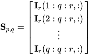
行列 P と Qは 完全シャッフル行列である。 [6] 完全シャッフル行列 S p , q は、 I r 単位行列のスライスをとることによって構築できます 。
ここで、
r
=
p
q
{\displaystyle r=pq}
S
p
,
q
=
[
I
r
(
1
:
q
:
r
,
:
)
I
r
(
2
:
q
:
r
,
:
)
⋮
I
r
(
q
:
q
:
r
,
:
)
]
{\displaystyle \mathbf {S} _{p,q}={\begin{bmatrix}\mathbf {I} _{r}(1:q:r,:)\\\mathbf {I} _{r}(2:q:r,:)\\\vdots \\\mathbf {I} _{r}(q:q:r,:)\end{bmatrix}}}
ここではMATLABの コロン表記法が部分行列を示すために使われており、 I rは r × r 単位行列である 。 そしての場合 、
A
∈
R
m
1
×
n
1
{\displaystyle \mathbf {A} \in \mathbb {R} ^{m_{1}\times n_{1}}}
B
∈
R
m
2
×
n
2
{\displaystyle \mathbf {B} \in \mathbb {R} ^{m_{2}\times n_{2}}}
B
⊗
A
=
S
m
1
,
m
2
(
A
⊗
B
)
S
n
1
,
n
2
T
{\displaystyle \mathbf {B} \otimes \mathbf {A} =\mathbf {S} _{m_{1},m_{2}}(\mathbf {A} \otimes \mathbf {B} )\mathbf {S} _{n_{1},n_{2}}^{\textsf {T}}}
混合積特性:
A 、 B 、 C 、 Dが 行列積 AC と BD を形成できる大きさの行列である 場合 、 [7]
(
A
⊗
B
)
(
C
⊗
D
)
=
(
A
C
)
⊗
(
B
D
)
.
{\displaystyle (\mathbf {A} \otimes \mathbf {B} )(\mathbf {C} \otimes \mathbf {D} )=(\mathbf {AC} )\otimes (\mathbf {BD} ).}
これは、通常の行列積とクロネッカー積が混合されているため、
混合積特性 と呼ばれます。
直接的な結果として(ここでも、 およびを考慮 )、
A
∈
R
m
1
×
n
1
{\displaystyle \mathbf {A} \in \mathbb {R} ^{m_{1}\times n_{1}}}
B
∈
R
m
2
×
n
2
{\displaystyle \mathbf {B} \in \mathbb {R} ^{m_{2}\times n_{2}}}
A
⊗
B
=
(
I
m
1
⊗
B
)
(
A
⊗
I
n
2
)
=
(
A
⊗
I
m
2
)
(
I
n
1
⊗
B
)
.
{\displaystyle \mathbf {A} \otimes \mathbf {B} =(\mathbf {I} _{m_{1}}\otimes \mathbf {B} )(\mathbf {A} \otimes \mathbf {I} _{n_{2}})=(\mathbf {A} \otimes \mathbf {I} _{m_{2}})(\mathbf {I} _{n_{1}}\otimes \mathbf {B} ).}
特に、 以下の
転置プロパティを使用すると、
A
=
Q
⊗
U
{\displaystyle \mathbf {A} =\mathbf {Q} \otimes \mathbf {U} }
Q と U が 直交 (または ユニタリ )であれば 、 A も 直交(またはユニタリ)します。
混合クロネッカー行列ベクトル積は次のように表すことができます。
(
A
⊗
B
)
vec
(
V
)
=
vec
(
B
V
A
T
)
{\displaystyle \left(\mathbf {A} \otimes \mathbf {B} \right)\operatorname {vec} \left(\mathbf {V} \right)=\operatorname {vec} (\mathbf {B} \mathbf {V} \mathbf {A} ^{T})}
ここで 、は ベクトル化 演算子に適用されます (行列の形状を変更することによって形成されます)。
vec
(
V
)
{\displaystyle \operatorname {vec} (\mathbf {V} )}
V
{\displaystyle \mathbf {V} }
アダマール積 (要素ごとの乗算):
混合積の性質は要素ごとの積にも当てはまる。A と C が 同じサイズの行列で、 B と Dも 同じサイズの行列であれば、 [7]
(
A
⊗
B
)
∘
(
C
⊗
D
)
=
(
A
∘
C
)
⊗
(
B
∘
D
)
.
{\displaystyle (\mathbf {A} \otimes \mathbf {B} )\circ (\mathbf {C} \otimes \mathbf {D} )=(\mathbf {A} \circ \mathbf {C} )\otimes (\mathbf {B} \circ \mathbf {D} ).}
クロネッカー積の逆関数:
したがって、 A ⊗ B が 逆であるのは、 A と B の 両方が逆である 場合に 限ります。この場合、逆は次のように表されます。
(
A
⊗
B
)
−
1
=
A
−
1
⊗
B
−
1
.
{\displaystyle (\mathbf {A} \otimes \mathbf {B} )^{-1}=\mathbf {A} ^{-1}\otimes \mathbf {B} ^{-1}.}
可逆積の性質は ムーア・ペンローズ擬似逆行列 にも成り立ち、 [7] [8]
すなわち
(
A
⊗
B
)
+
=
A
+
⊗
B
+
.
{\displaystyle (\mathbf {A} \otimes \mathbf {B} )^{+}=\mathbf {A} ^{+}\otimes \mathbf {B} ^{+}.}
圏論 の言語では 、クロネッカー積(およびより一般的なテンソル積)の混合積特性は、 体 F 上の行列の圏 Mat F が実際には モノイド圏 であり、対象が自然数 n であり、射 n → m がFに要素を持つ n × m 行列で あり 、合成が行列の乗算で与えられ、恒等射が単に n × n 恒等行列 I n であり、テンソル積がクロネッカー積で与えられることを示しています。 [9]
Mat F は、 F 上の有限次元ベクトル空間の 同値カテゴリ FinVect F の具体的な スケルトンカテゴリ であり 、その対象はそのような有限次元ベクトル空間 V 、矢印は F 線型写像 L : V → W 、恒等矢印は空間の恒等写像です。カテゴリの同値性は、 F 上の すべての有限次元ベクトル空間 Vで 基底を同時に選択する ことに相当します。行列の要素は、選択された基底に関するこれらのマッピングを表します。同様に、クロネッカー積は、 選択された基底における テンソル積の表現です。 転置 :
転置と 共役転置は クロネッカー積に対して分配的である:
(
A
⊗
B
)
T
=
A
T
⊗
B
T
{\displaystyle (\mathbf {A} \otimes \mathbf {B} )^{\textsf {T}}=\mathbf {A} ^{\textsf {T}}\otimes \mathbf {B} ^{\textsf {T}}}
そして
(
A
⊗
B
)
∗
=
A
∗
⊗
B
∗
.
{\displaystyle (\mathbf {A} \otimes \mathbf {B} )^{*}=\mathbf {A} ^{*}\otimes \mathbf {B} ^{*}.}
決定要因 :
A を n × n 行列、 Bを m × m 行列と します 。すると
|
A
⊗
B
|
=
|
A
|
m
|
B
|
n
.
{\displaystyle \left|\mathbf {A} \otimes \mathbf {B} \right|=\left|\mathbf {A} \right|^{m}\left|\mathbf {B} \right|^{n}.}
| A |
の指数は B の位数であり、 | B |の指数は A の位数です 。 クロネッカー和と 累乗 :
A が n × n 、 B が m × m 、 I kが k × k 単位行列 を表す 場合、 クロネッカー和 と
呼ばれるものを次のように定義できます。
A
⊕
B
=
A
⊗
I
m
+
I
n
⊗
B
.
{\displaystyle \mathbf {A} \oplus \mathbf {B} =\mathbf {A} \otimes \mathbf {I} _{m}+\mathbf {I} _{n}\otimes \mathbf {B} .}
これは、 2 つの行列の 直和 とは 異なります。この演算は、 リー代数 上のテンソル積に関連しており、詳細は、以下の「抽象 テンソル積 との関係」の項 (#抽象プロパティ) で説明します 。
行列指数関数 には次のような式があり 、これはいくつかの数値評価に有用である。 [10]
exp
(
N
⊕
M
)
=
exp
(
N
)
⊗
exp
(
M
)
{\displaystyle \exp({\mathbf {N} \oplus \mathbf {M} })=\exp(\mathbf {N} )\otimes \exp(\mathbf {M} )}
クロネッカー和は、 相互作用しない システムの集団を考えるとき、 物理学 において自然に現れる。 [ 要出典 ] H k を k 番目のそのようなシステムのハミルトニアンと する 。すると、集団の全ハミルトニアンは
H
Tot
=
⨁
k
H
k
.
{\displaystyle H_{\operatorname {Tot} }=\bigoplus _{k}H^{k}.}
クロネッカー積の ベクトル化:
を行列 、を 行列と します 。クロネッカー積とベクトル化の順序を入れ替えると、2 つの演算は 交換行列 、 を含む関数 を介して線形にリンクできます。 つまり、 と は 次の関係を持ちます。
A
{\displaystyle A}
m
×
n
{\displaystyle m\times n}
B
{\displaystyle B}
p
×
q
{\displaystyle p\times q}
K
q
m
{\displaystyle K_{qm}}
vec
(
Kron
(
A
,
B
)
)
{\displaystyle \operatorname {vec} (\operatorname {Kron} (A,B))}
Kron
(
vec
A
,
vec
B
)
{\displaystyle \operatorname {Kron} (\operatorname {vec} A,\operatorname {vec} B)}
vec
(
A
⊗
B
)
=
(
I
n
⊗
K
q
m
⊗
I
p
)
(
vec
A
⊗
vec
B
)
.
{\displaystyle \operatorname {vec} (A\otimes B)=(I_{n}\otimes K_{qm}\otimes I_{p})(\operatorname {vec} A\otimes \operatorname {vec} B).}
さらに、上記の関係は 、またはのいずれかの観点から 次のように並べ替えることができます。
vec
A
{\displaystyle \operatorname {vec} A}
vec
B
{\displaystyle \operatorname {vec} B}
vec
(
A
⊗
B
)
=
(
I
n
⊗
G
)
vec
A
=
(
H
⊗
I
p
)
vec
B
,
{\displaystyle \operatorname {vec} (A\otimes B)=(I_{n}\otimes G)\operatorname {vec} A=(H\otimes I_{p})\operatorname {vec} B,}
どこ
G
=
(
K
q
m
⊗
I
p
)
(
I
m
⊗
vec
B
)
and
H
=
(
I
n
⊗
K
q
m
)
(
vec
A
⊗
I
q
)
.
{\displaystyle G=(K_{qm}\otimes I_{p})(I_{m}\otimes \operatorname {vec} B){\text{ and }}H=(I_{n}\otimes K_{qm})(\operatorname {vec} A\otimes I_{q}).}
外積 :
と が任意のベクトルである
場合、 と の間の外積は と定義されます 。クロネッカー積は、外積と次の式で関連しています 。
x
∈
R
n
{\displaystyle x\in \mathbb {R} ^{n}}
y
∈
R
m
{\displaystyle y\in \mathbb {R} ^{m}}
x
{\displaystyle x}
y
{\displaystyle y}
x
y
T
{\displaystyle xy^{T}}
y
⊗
x
=
vec
(
x
y
T
)
{\displaystyle y\otimes x=\operatorname {vec} (xy^{T})}
抽象プロパティ スペクトラム :
A と B が それぞれ n と m の 大きさの正方行列である とする。λ 1 , ..., λ n を A の 固有値とし 、 μ 1 , ..., μ m を B の 固有値 とする( 重複度 順に並べる)。すると、 A ⊗ B の 固有値は 次のように なる
。
λ
i
μ
j
,
i
=
1
,
…
,
n
,
j
=
1
,
…
,
m
.
{\displaystyle \lambda _{i}\mu _{j},\qquad i=1,\ldots ,n,\,j=1,\ldots ,m.}
クロネッカー積の
トレース と 行列式 は次のように与えられる。
tr
(
A
⊗
B
)
=
tr
A
tr
B
and
det
(
A
⊗
B
)
=
(
det
A
)
m
(
det
B
)
n
.
{\displaystyle \operatorname {tr} (\mathbf {A} \otimes \mathbf {B} )=\operatorname {tr} \mathbf {A} \,\operatorname {tr} \mathbf {B} \quad {\text{and}}\quad \det(\mathbf {A} \otimes \mathbf {B} )=(\det \mathbf {A} )^{m}(\det \mathbf {B} )^{n}.}
特異値 :
A と Bが 長方形行列である場合 、それらの 特異値 を考えることができる。Aが r A 個の 非ゼロ特異値を持つと仮定する 。すなわち、
σ
A
,
i
,
i
=
1
,
…
,
r
A
.
{\displaystyle \sigma _{\mathbf {A} ,i},\qquad i=1,\ldots ,r_{\mathbf {A} }.}
同様に、 B の非ゼロ特異値を 次のように
表す。
σ
B
,
i
,
i
=
1
,
…
,
r
B
.
{\displaystyle \sigma _{\mathbf {B} ,i},\qquad i=1,\ldots ,r_{\mathbf {B} }.}
するとクロネッカー積 A ⊗ Bは r A r Bの 非零特異値を持ち 、すなわち
σ
A
,
i
σ
B
,
j
,
i
=
1
,
…
,
r
A
,
j
=
1
,
…
,
r
B
.
{\displaystyle \sigma _{\mathbf {A} ,i}\sigma _{\mathbf {B} ,j},\qquad i=1,\ldots ,r_{\mathbf {A} },\,j=1,\ldots ,r_{\mathbf {B} }.}
行列の階数は 非ゼロ特異値の数に等しい
ので、
rank
(
A
⊗
B
)
=
rank
A
rank
B
.
{\displaystyle \operatorname {rank} (\mathbf {A} \otimes \mathbf {B} )=\operatorname {rank} \mathbf {A} \,\operatorname {rank} \mathbf {B} .}
抽象 テンソル積 との関係:
行列のクロネッカー積は、線形写像の抽象テンソル積に対応します。具体的には、ベクトル空間 V 、 W 、 X 、 Y がそれぞれ基底 { v 1 、 ...、 v m }、 { w 1 、 ...、 w n }、 { x 1 、 ...、 x d }、 { y 1 、 ...、 y e } を持ち、行列 A と B が それぞれ適切な基底での線形変換 S : V → X と T : W → Y を 表す場合、行列 A ⊗ B は 、 V ⊗ W の基底 { v 1 ⊗ w 1 、 v 1 ⊗ w 2 、 ...、 v 2 ⊗ w 1 、 ...、 v m ⊗ w n }と、 同様 に定義された X ⊗ Y の基底に関する 2 つ の 写像S ⊗ T : V ⊗ W → X ⊗ Y の テンソル 積 を 表し、 A ⊗ B ( v i ⊗ w j ) = ( Av i ) ⊗ ( Bw j ) 、ここで i と jは 適切な範囲の整数である。 [11]
V と W が リー代数 で 、 S : V → V と T : W → W がリー代数準同型 である
とき、 A と B のクロネッカー和は 誘導リー代数準同型 V ⊗ W → V ⊗ W を表す。 [ 出典が必要 ] グラフの積 との関係 :
2つの グラフの 隣接行列
のクロネッカー積は、 テンソル積グラフ の隣接行列である 。2つの グラフの隣接行列のクロネッカー和は 、直積グラフ の隣接行列である 。 [12]
行列方程式 クロネッカー積は、いくつかの行列方程式の便利な表現を得るために使用できます。たとえば、方程式 AXB = C を 考えてみましょう。ここで、 A 、 B 、 C は与えられた行列で、行列 X は 未知数です。「vec トリック」を使用して、この方程式を次のように書き直すことができます。
(
B
T
⊗
A
)
vec
(
X
)
=
vec
(
A
X
B
)
=
vec
(
C
)
.
{\displaystyle \left(\mathbf {B} ^{\textsf {T}}\otimes \mathbf {A} \right)\,\operatorname {vec} (\mathbf {X} )=\operatorname {vec} (\mathbf {AXB} )=\operatorname {vec} (\mathbf {C} ).}
ここで、vec( X )は行列 Xの ベクトル化 を表し、 X の列を1つの 列ベクトル に積み重ねることによって形成されます 。
クロネッカー積の特性から、 A と B が可逆である
場合に限り、方程式 AXB = C は一意の解を持つことがわかります (Horn & Johnson 1991、補題 4.3.1)。
X と C が それぞれ列ベクトル u と v に行順に並べられている場合 、(Jain 1989、2.8 ブロック行列とクロネッカー積)
v
=
(
A
⊗
B
T
)
u
.
{\displaystyle \mathbf {v} =\left(\mathbf {A} \otimes \mathbf {B} ^{\textsf {T}}\right)\mathbf {u} .}
その理由は
v
=
vec
(
(
A
X
B
)
T
)
=
vec
(
B
T
X
T
A
T
)
=
(
A
⊗
B
T
)
vec
(
X
T
)
=
(
A
⊗
B
T
)
u
.
{\displaystyle \mathbf {v} =\operatorname {vec} \left((\mathbf {AXB} )^{\textsf {T}}\right)=\operatorname {vec} \left(\mathbf {B} ^{\textsf {T}}\mathbf {X} ^{\textsf {T}}\mathbf {A} ^{\textsf {T}}\right)=\left(\mathbf {A} \otimes \mathbf {B} ^{\textsf {T}}\right)\operatorname {vec} \left(\mathbf {X^{\textsf {T}}} \right)=\left(\mathbf {A} \otimes \mathbf {B} ^{\textsf {T}}\right)\mathbf {u} .}
アプリケーション この公式の応用例については、 リアプノフ方程式に関する記事を参照してください。この公式は、 行列正規分布が 多変量正規分布 の特殊なケースである ことを示すのにも役立ちます。この公式は、2D 画像処理 操作を行列ベクトル形式で
表すのにも役立ちます。
もう 1 つの例は、行列をクロネッカー積として因数分解できる場合です。この場合、上記の式を使用して行列の乗算をより高速に実行できます。これは、 基数 2 の FFT や 高速ウォルシュ アダマール変換 で行われるように、再帰的に適用できます。既知の行列を 2 つの小さな行列のクロネッカー積に分割することは、「最も近いクロネッカー積」問題として知られており、 SVD を 使用して正確に解決できます [13] 。最適な方法で行列を 2 つ以上の行列のクロネッカー積に分割することは困難な問題であり、現在も研究が進められています。一部の著者は、これをテンソル分解問題として扱っています。 [14] [15]
最小二乗法 と組み合わせることで 、クロネッカー積は 手と目の較正問題 に対する正確な解として使用することができます。 [16]
関連する 2 つの 行列演算は、 分割された行列 に対して演算される Tracy–Singh 積 と Khatri–Rao 積 です。m × n 行列 Aを m i × n j ブロック A ij に分割し 、 p × q 行列 B を p k × q ℓ ブロック B kl に分割する とします。ここで、もちろん Σ i m i = m 、 Σ j n j = n 、 Σ k p k = p 、 Σ ℓ q ℓ = q です。
トレイシー・シン積 トレイシー ・シン積は 次のように定義される [17] [18] [19]
A
∘
B
=
(
A
i
j
∘
B
)
i
j
=
(
(
A
i
j
⊗
B
k
l
)
k
l
)
i
j
{\displaystyle \mathbf {A} \circ \mathbf {B} =\left(\mathbf {A} _{ij}\circ \mathbf {B} \right)_{ij}=\left(\left(\mathbf {A} _{ij}\otimes \mathbf {B} _{kl}\right)_{kl}\right)_{ij}}
これは、 mp × nq 積 A B の( ij )番目のサブブロックが m i p × n j q 行列 A ij B であり 、その( kℓ )番目のサブブロックが m i p k × n j q ℓ 行列 A ij ⊗ B kℓ に等しいことを意味します。本質的に、Tracy-Singh積は、2つの行列の各パーティションのペアごとのクロネッカー積です。
∘
{\displaystyle \circ }
∘
{\displaystyle \circ }
たとえば、 A と B が 両方とも 2 × 2 に分割された行列の場合、次のようになります。
A
=
[
A
11
A
12
A
21
A
22
]
=
[
1
2
3
4
5
6
7
8
9
]
,
B
=
[
B
11
B
12
B
21
B
22
]
=
[
1
4
7
2
5
8
3
6
9
]
,
{\displaystyle \mathbf {A} =\left[{\begin{array}{c | c}\mathbf {A} _{11}&\mathbf {A} _{12}\\\hline \mathbf {A} _{21}&\mathbf {A} _{22}\end{array}}\right]=\left[{\begin{array}{c c | c}1&2&3\\4&5&6\\\hline 7&8&9\end{array}}\right],\quad \mathbf {B} =\left[{\begin{array}{c | c}\mathbf {B} _{11}&\mathbf {B} _{12}\\\hline \mathbf {B} _{21}&\mathbf {B} _{22}\end{array}}\right]=\left[{\begin{array}{c | c c}1&4&7\\\hline 2&5&8\\3&6&9\end{array}}\right],}
結果は次のようになります:
A
∘
B
=
[
A
11
∘
B
A
12
∘
B
A
21
∘
B
A
22
∘
B
]
=
[
A
11
⊗
B
11
A
11
⊗
B
12
A
12
⊗
B
11
A
12
⊗
B
12
A
11
⊗
B
21
A
11
⊗
B
22
A
12
⊗
B
21
A
12
⊗
B
22
A
21
⊗
B
11
A
21
⊗
B
12
A
22
⊗
B
11
A
22
⊗
B
12
A
21
⊗
B
21
A
21
⊗
B
22
A
22
⊗
B
21
A
22
⊗
B
22
]
=
[
1
2
4
7
8
14
3
12
21
4
5
16
28
20
35
6
24
42
2
4
5
8
10
16
6
15
24
3
6
6
9
12
18
9
18
27
8
10
20
32
25
40
12
30
48
12
15
24
36
30
45
18
36
54
7
8
28
49
32
56
9
36
63
14
16
35
56
40
64
18
45
72
21
24
42
63
48
72
27
54
81
]
.
{\displaystyle {\begin{aligned}\mathbf {A} \circ \mathbf {B} ={}&\left[{\begin{array}{c | c}\mathbf {A} _{11}\circ \mathbf {B} &\mathbf {A} _{12}\circ \mathbf {B} \\\hline \mathbf {A} _{21}\circ \mathbf {B} &\mathbf {A} _{22}\circ \mathbf {B} \end{array}}\right]\\={}&\left[{\begin{array}{c | c | c | c}\mathbf {A} _{11}\otimes \mathbf {B} _{11}&\mathbf {A} _{11}\otimes \mathbf {B} _{12}&\mathbf {A} _{12}\otimes \mathbf {B} _{11}&\mathbf {A} _{12}\otimes \mathbf {B} _{12}\\\hline \mathbf {A} _{11}\otimes \mathbf {B} _{21}&\mathbf {A} _{11}\otimes \mathbf {B} _{22}&\mathbf {A} _{12}\otimes \mathbf {B} _{21}&\mathbf {A} _{12}\otimes \mathbf {B} _{22}\\\hline \mathbf {A} _{21}\otimes \mathbf {B} _{11}&\mathbf {A} _{21}\otimes \mathbf {B} _{12}&\mathbf {A} _{22}\otimes \mathbf {B} _{11}&\mathbf {A} _{22}\otimes \mathbf {B} _{12}\\\hline \mathbf {A} _{21}\otimes \mathbf {B} _{21}&\mathbf {A} _{21}\otimes \mathbf {B} _{22}&\mathbf {A} _{22}\otimes \mathbf {B} _{21}&\mathbf {A} _{22}\otimes \mathbf {B} _{22}\end{array}}\right]\\={}&\left[{\begin{array}{c c | c c c c | c | c c}1&2&4&7&8&14&3&12&21\\4&5&16&28&20&35&6&24&42\\\hline 2&4&5&8&10&16&6&15&24\\3&6&6&9&12&18&9&18&27\\8&10&20&32&25&40&12&30&48\\12&15&24&36&30&45&18&36&54\\\hline 7&8&28&49&32&56&9&36&63\\\hline 14&16&35&56&40&64&18&45&72\\21&24&42&63&48&72&27&54&81\end{array}}\right].\end{aligned}}}
カトリ・ラオ積
顔を割る製品 混合製品の特性 [20]
A
⊗
(
B
∙
C
)
=
(
A
⊗
B
)
∙
C
,
{\displaystyle \mathbf {A} \otimes (\mathbf {B} \bullet \mathbf {C} )=(\mathbf {A} \otimes \mathbf {B} )\bullet \mathbf {C} ,}
ここで は 面分割積 を表す 。 [21] [22]
∙
{\displaystyle \bullet }
(
A
∙
B
)
(
C
⊗
D
)
=
(
A
C
)
∙
(
B
D
)
,
{\displaystyle (\mathbf {A} \bullet \mathbf {B} )(\mathbf {C} \otimes \mathbf {D} )=(\mathbf {A} \mathbf {C} )\bullet (\mathbf {B} \mathbf {D} ),}
同様に: [23]
(
A
∙
L
)
(
B
⊗
M
)
⋯
(
C
⊗
S
)
=
(
A
B
⋯
C
)
∙
(
L
M
⋯
S
)
,
{\displaystyle (\mathbf {A} \bullet \mathbf {L} )(\mathbf {B} \otimes \mathbf {M} )\cdots (\mathbf {C} \otimes \mathbf {S} )=(\mathbf {A} \mathbf {B} \cdots \mathbf {C} )\bullet (\mathbf {L} \mathbf {M} \cdots \mathbf {S} ),}
c
T
∙
d
T
=
c
T
⊗
d
T
,
{\displaystyle \mathbf {c} ^{\textsf {T}}\bullet \mathbf {d} ^{\textsf {T}}=\mathbf {c} ^{\textsf {T}}\otimes \mathbf {d} ^{\textsf {T}},}
ここで、 およびは ベクトル である 。 [24]
c
{\displaystyle \mathbf {c} }
d
{\displaystyle \mathbf {d} }
(
A
∙
B
)
(
c
⊗
d
)
=
(
A
c
)
∘
(
B
d
)
,
{\displaystyle (\mathbf {A} \bullet \mathbf {B} )(\mathbf {c} \otimes \mathbf {d} )=(\mathbf {A} \mathbf {c} )\circ (\mathbf {B} \mathbf {d} ),}
ここで 、 と は ベクトル であり 、 は アダマール積 を表します 。
c
{\displaystyle \mathbf {c} }
d
{\displaystyle \mathbf {d} }
∘
{\displaystyle \circ }
同様に:
(
A
∙
B
)
(
M
N
c
⊗
Q
P
d
)
=
(
A
M
N
c
)
∘
(
B
Q
P
d
)
,
{\displaystyle (\mathbf {A} \bullet \mathbf {B} )(\mathbf {M} \mathbf {N} \mathbf {c} \otimes \mathbf {Q} \mathbf {P} \mathbf {d} )=(\mathbf {A} \mathbf {M} \mathbf {N} \mathbf {c} )\circ (\mathbf {B} \mathbf {Q} \mathbf {P} \mathbf {d} ),}
F
(
C
(
1
)
x
⋆
C
(
2
)
y
)
=
(
F
C
(
1
)
∙
F
C
(
2
)
)
(
x
⊗
y
)
=
F
C
(
1
)
x
∘
F
C
(
2
)
y
,
{\displaystyle {\mathcal {F}}(C^{(1)}x\star C^{(2)}y)=({\mathcal {F}}C^{(1)}\bullet {\mathcal {F}}C^{(2)})(x\otimes y)={\mathcal {F}}C^{(1)}x\circ {\mathcal {F}}C^{(2)}y,}
ここで、 はベクトル 畳み込み であり、は フーリエ変換行列 である(この結果は カウントスケッチ 特性 の進化である [25] )、 [21] [22]
⋆
{\displaystyle \star }
F
{\displaystyle {\mathcal {F}}}
(
A
∙
L
)
(
B
⊗
M
)
⋯
(
C
⊗
S
)
(
K
∗
T
)
=
(
A
B
⋅
C
K
)
∘
(
L
M
⋯
S
T
)
,
{\displaystyle (\mathbf {A} \bullet \mathbf {L} )(\mathbf {B} \otimes \mathbf {M} )\cdots (\mathbf {C} \otimes \mathbf {S} )(\mathbf {K} \ast \mathbf {T} )=(\mathbf {A} \mathbf {B} \cdot \mathbf {C} \mathbf {K} )\circ (\mathbf {L} \mathbf {M} \cdots \mathbf {S} \mathbf {T} ),}
ここで、 は 列方向のカトリ・ラオ積 を表します 。
∗
{\displaystyle \ast }
同様に:
(
A
∙
L
)
(
B
⊗
M
)
⋯
(
C
⊗
S
)
(
c
⊗
d
)
=
(
A
B
⋯
C
c
)
∘
(
L
M
⋯
S
d
)
,
{\displaystyle (\mathbf {A} \bullet \mathbf {L} )(\mathbf {B} \otimes \mathbf {M} )\cdots (\mathbf {C} \otimes \mathbf {S} )(c\otimes d)=(\mathbf {A} \mathbf {B} \cdots \mathbf {C} \mathbf {c} )\circ (\mathbf {L} \mathbf {M} \cdots \mathbf {S} \mathbf {d} ),}
(
A
∙
L
)
(
B
⊗
M
)
⋯
(
C
⊗
S
)
(
P
c
⊗
Q
d
)
=
(
A
B
⋯
C
P
c
)
∘
(
L
M
⋯
S
Q
d
)
,
{\displaystyle (\mathbf {A} \bullet \mathbf {L} )(\mathbf {B} \otimes \mathbf {M} )\cdots (\mathbf {C} \otimes \mathbf {S} )(\mathbf {P} \mathbf {c} \otimes \mathbf {Q} \mathbf {d} )=(\mathbf {A} \mathbf {B} \cdots \mathbf {C} \mathbf {P} \mathbf {c} )\circ (\mathbf {L} \mathbf {M} \cdots \mathbf {S} \mathbf {Q} \mathbf {d} ),}
ここで 、 およびは ベクトル です 。
c
{\displaystyle \mathbf {c} }
d
{\displaystyle \mathbf {d} }
参照
注記
^ Weisstein, Eric W. 「クロネッカー積」。mathworld.wolfram.com . 2020年9月6日 閲覧 。
^ Zehfuss、G. (1858)。 「Ueber eine gewisse Determinante」。 数学と物理学の時代 。 3 : 298–301。
^ヘンダーソン、ハロルド V.; プケルスハイム、フリードリヒ; サール 、シェイル R. (1983)。「クロネッカー積の歴史について」。 線形および多重線形代数 。14 ( 2): 113–120。doi : 10.1080/03081088308817548。hdl : 1813 /32834。ISSN 0308-1087 。 ^ Sayed, Ali H. (2022-12-22). データからの推論と学習:基礎。ケンブリッジ大学出版局 。ISBN 978-1-009-21812-2 。 ^ Henderson, HV; Searle, SR (1980). 「vec-permutation行列、vec演算子、およびクロネッカー積:レビュー」 (PDF) . 線形および多重線形代数 . 9 (4): 271–288. doi :10.1080/03081088108817379. hdl : 1813/32747 .
^ Van Loan, Charles F. (2000). 「ユビキタス・クロネッカー積」. 計算および応用数学ジャーナル . 123 (1–2): 85–100. Bibcode :2000JCoAM.123...85L. doi : 10.1016/s0377-0427(00)00393-9 .
^ abc Liu, Shuangzhe; Trenkler, Götz; Kollo, Tõnu; von Rosen, Dietrich; Baksalary, Oskar Maria (2023). 「ハインツ・ノイデッカー教授と行列微分計算」. 統計論文 . 65 (4): 2605–2639. doi :10.1007/s00362-023-01499-w. ^ Langville, Amy N. ; Stewart, William J. (2004 年 6 月 1 日). 「クロネッカー積と確率オートマトンネットワーク」. Journal of Computational and Applied Mathematics . 167 (2): 429–447. Bibcode :2004JCoAM.167..429L. doi : 10.1016/j.cam.2003.10.010 .
^ マセド、ヒューゴ・ダニエル;オリベイラ、ホセ・ヌーノ (2013)。 「線形代数の型付け: 双積指向のアプローチ」。 コンピュータプログラミングの科学 。 78 (11): 2160–2191。 arXiv : 1312.4818 。 Bibcode :2013arXiv1312.4818M。 CiteSeerX 10.1.1.747.2083 。 土井 :10.1016/j.scico.2012.07.012。 S2CID 9846072。
^ Brewer, JW (1969). 「クロネッカー行列積と行列方程式システムに関する注記」 SIAM Journal on Applied Mathematics . 17 (3): 603–606. doi :10.1137/0117057.
^
^ Knuth, DE「Pre-Fascicle 0a: Introduction to Combinatorial Algorithms」(第0刷、第2版)を参照 。演習96の解答。2019年5月13日時点のオリジナルよりアーカイブ。 2007年10月24日 閲覧 。 Knuth, DE The Art of Computer Programming . Vol. 4A の一部として掲載されます。 ^ Van Loan, C.; Pitsianis, N. (1992). クロネッカー積による近似 。イサカ、ニューヨーク:コーネル大学出版局。
^ King Keung Wu、Yam, Yeung、Meng, Helen、Mesbahi, Mehran (2016)。「テンソル積アルゴリズムによる多重因子行列のクロネッカー積近似」。2016 IEEE 国際システム・人間・サイバネティクス会議 (SMC) 。pp. 004277–004282。doi : 10.1109 / SMC.2016.7844903。ISBN
978-1-5090-1897-0 . S2CID 30695585。
^ Dantas, Cássio F.; Cohen, Jérémy E.; Gribonval, Rémi (2018). 「低ランクテンソル分解を用いたスパース表現の高速辞書の学習」。潜在変数分析と信号分離 (PDF) 。コンピュータサイエンスの講義ノート。第 10891 巻。pp. 456–466。doi : 10.1007 / 978-3-319-93764-9_42。ISBN
978-3-319-93763-2 . S2CID 46963798。
^ Li, Algo; et al. (2010年9月4日). 「デュアルクォータニオンとクロネッカー積を使用したロボットワールドとハンドアイの同時キャリブレーション」 (PDF) 。 International Journal of the Physical Sciences 。 5 (10): 1530–1536. S2CID 7446157. 2020年2月9日時点のオリジナル (PDF) からアーカイブ。
^ Tracy, DS; Singh, RP (1972). 「新しい行列積と行列微分化への応用」. Statistica Neerlandica . 26 (4): 143–157. doi :10.1111/j.1467-9574.1972.tb00199.x.
^ Liu, Shuangzhe (1999). 「Khatri–Rao積とTracy–Singh積の行列結果」. 線形代数とその応用 . 289 (1–3): 267–277. doi : 10.1016/S0024-3795(98)10209-4 .
^ Liu, Shuangzhe; Trenkler, Götz (2008). 「アダマール、カトリ・ラオ、クロネッカーおよびその他の行列積」. 国際情報システム科学ジャーナル . 4 (1): 160–177.
^ Slyusar, VI (1998) [1996年12月27日]. 「レーダーアプリケーションにおけるマトリックスの最終製品」 (PDF) . 無線エレクトロニクスおよび通信システム . 41 (3): 50–53.
^ ab Slyusar, Vadym (1999). 「DSP の新しい行列演算」(自費出版の講義)。doi :10.13140/RG.2.2.31620.76164/1 – ResearchGate 経由 。
^ ab Slyusar, VI (1998 年 3 月 13 日). 「行列の面積のファミリーとその特性」 (PDF) . サイバネティクスとシステム分析 C/C of Kibernetika I Sistemnyi Analiz. 1999 . 35 (3): 379–384. doi :10.1007/BF02733426. S2CID 119661450.
^ Slyusar, VI (1997-09-15). レーダー応用のための行列積の新しい演算 (PDF) . 電磁波および音波理論の直接問題と逆問題 (DIPED-97)、リヴィウ。pp. 73–74。
^ アーレ、トーマス・ディブダール;クヌッセン、ヤコブ・ベク・テイス(2019-09-03)。 「ほぼ最適なテンソル スケッチ」。 arXiv : 1909.01821 [cs.DS]。
^ Ninh , Pham; Pagh, Rasmus (2013). 明示的な特徴マップによる高速でスケーラブルな多項式カーネル 。知識発見とデータマイニングに関する SIGKDD 国際会議。Association for Computing Machinery。CiteSeerX 10.1.1.718.2766。doi : 10.1145 /2487575.2487591。
参考文献 ホーン、ロジャー A. ; ジョンソン、チャールズ R. (1991)。行列分析のトピック。ケンブリッジ大学出版局 。ISBN 978-0-521-46713-1 。 Jain, Anil K. (1989). デジタル画像処理の基礎. Prentice Hall. Bibcode :1989fdip.book.....J. ISBN 978-0-13-336165-0 。 Steeb, Willi-Hans (1997)。 行列計算とクロネッカー積とその応用および C++ プログラム 。World Scientific Publishing。ISBN 978-981-02-3241-2 。 Steeb, Willi-Hans (2006)。初級および上級行列計算 の問題と解答。World Scientific Publishing。ISBN 978-981-256-916-5 。 Liu, Shuangzhe、Trenkler, Götz (2008)、「アダマール、カトリ・ラオ、クロネッカーおよびその他の行列積」、 International Journal of Information and Systems Sciences 、 4 : 160–177
外部リンク 「テンソル積」、 数学百科事典 、 EMS Press 、2001 [1994] 「クロネッカー製品」。 プラネットマス 。 「クロネッカー積」 。MathWorld 。 「新しいクロネッカー積問題」 (PDF) 。 「最も古い使用例」。 クロネッカー行列、ゼフス行列、または直積行列のエントリには、歴史的な情報があります。 2 つの行列のクロネッカー積を計算します。SourceForge ( 汎用 C++ および Fortran 90 ソース コード)。2015-06-27。 「クロネッカー積」。RosettaCode.org . 2020年12月31日. 2021年1月13日 閲覧 。 40 以上の言語で提供されるソフトウェア ソース。







![{\displaystyle {\begin{bmatrix}1&2\\3&4\\\end{bmatrix}}\otimes {\begin{bmatrix}0&5\\6&7\\\end{bmatrix}}={\begin{bmatrix}1{\begin{bmatrix}0&5\\6&7\\\end{bmatrix}}&2{\begin{bmatrix}0&5\\6&7\\\end{bmatrix}}\\3{\begin{bmatrix}0&5\\6&7\\\end{bmatrix}}&4{\begin{bmatrix}0&5\\6&7\\\end{bmatrix}}\\\end{bmatrix}}=\left[{\begin{array}{cc|cc}1\times 0&1\times 5&2\times 0&2\times 5\\1\times 6&1\times 7&2\times 6&2\times 7\\\hline 3\times 0&3\times 5&4\times 0&4\times 5\\3\times 6&3\times 7&4\times 6&4\times 7\\\end{array}}\right]=\left[{\begin{array}{cc|cc}0&5&0&10\\6&7&12&14\\\hline 0&15&0&20\\18&21&24&28\end{array}}\right].}](https://wikimedia.org/api/rest_v1/media/math/render/svg/74fc4867467d053ae700ebb040ddfbe42600288c)
![{\displaystyle {\begin{bmatrix}1&-4&7\\-2&3&3\end{bmatrix}}\otimes {\begin{bmatrix}8&-9&-6&5\\1&-3&-4&7\\2&8&-8&-3\\1&2&-5&-1\end{bmatrix}}=\left[{\begin{array}{cccc|cccc|cccc}8&-9&-6&5&-32&36&24&-20&56&-63&-42&35\\1&-3&-4&7&-4&12&16&-28&7&-21&-28&49\\2&8&-8&-3&-8&-32&32&12&14&56&-56&-21\\1&2&-5&-1&-4&-8&20&4&7&14&-35&-7\\\hline -16&18&12&-10&24&-27&-18&15&24&-27&-18&15\\-2&6&8&-14&3&-9&-12&21&3&-9&-12&21\\-4&-16&16&6&6&24&-24&-9&6&24&-24&-9\\-2&-4&10&2&3&6&-15&-3&3&6&-15&-3\end{array}}\right]}](https://wikimedia.org/api/rest_v1/media/math/render/svg/1d5453c59a261174eb2458c21ff9bdd30dc2c87d)



































![{\displaystyle \mathbf {A} =\left[{\begin{array}{c | c}\mathbf {A} _{11}&\mathbf {A} _{12}\\\hline \mathbf {A} _{21}&\mathbf {A} _{22}\end{array}}\right]=\left[{\begin{array}{cc | c}1&2&3\\4&5&6\\\hline 7&8&9\end{array}}\right],\quad \mathbf {B} =\left[{\begin{array}{c | c}\mathbf {B} _{11}&\mathbf {B} _{12}\\\hline \mathbf {B} _{21}&\mathbf {B} _{22}\end{array}}\right]=\left[{\begin{array}{c | cc}1&4&7\\\hline 2&5&8\\3&6&9\end{array}}\right],}](https://wikimedia.org/api/rest_v1/media/math/render/svg/a53cde028551100b310943f25b2028a764436687)
![{\displaystyle {\begin{aligned}\mathbf {A} \circ \mathbf {B} ={}&\left[{\begin{array}{c | c}\mathbf {A} _{11}\circ \mathbf {B} &\mathbf {A} _{12}\circ \mathbf {B} \\\hline \mathbf {A} _{21}\circ \mathbf {B} &\mathbf {A} _{22}\circ \mathbf {B} \end{配列}}\right]\\={}&\left[{\begin{配列}{c | c | c | c}\mathbf {A} _{11}\otimes \mathbf {B} _{11}&\mathbf {A} _{11}\otimes \mathbf {B} _{12}&\mathbf {A} _ {12}\otimes \mathbf {B} _{11}&\mathbf {A} _{12}\otimes \mathbf {B} _{12}\\\hline \mathbf {A} _{11}\otimes \mathbf {B} _{21}&\mathbf {A} _{11}\otimes \mathbf {B} _{ 22}&\mathbf {A} _{12}\otimes \mathbf {B} _{21}&\mathbf {A} _{12}\otimes \mathbf {B} _{22}\\\hline \mathbf {A} _{21}\otimes \mathbf {B} _{11}& \mathbf {A} _{21}\otimes \mathbf {B} _{12}&\mathbf {A} _{22}\otimes \mathbf {B} _{11}&\mathbf {A} _{22}\otimes \mathbf {B} _{12}\\\hline \mathbf {A} _{21}\ otimes \mathbf {B} _{21}&\mathbf {A} _{21}\otimes \mathbf {B} _{22}&\mathbf {A} _{22}\otimes \mathbf {B} _{21}&\mathbf {A} _{22}\otimes \mathbf {B} _{22}\ end{array}}\right]\\={}&\left[{\begin{array}{cc | CCCC | c | cc}1&2&4&7&8&14&3&12&21\\4&5&16&28&20&35&6&24&42\\\hline 2&4&5&8&10&16&6&15&24\\3&6&6&9&12&18&9&18&27\\8&10&20&32&25&40&12&30&48\\12&15&24&36&30&45&18&36&54\\\hline 7&8&28&49&32&56&9&36&63\\\hライン14&16&35&56&40&64&18&45&72\\21&24&42&63&48&72&27&54&81\end{配列}}\right].\end{整列}}}](https://wikimedia.org/api/rest_v1/media/math/render/svg/a9db8d2cd6699bcf107b36674a3542ca635e19ff)














