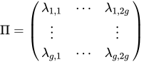
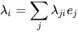
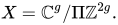
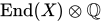
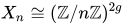
複素トーラスの周期行列 g 次元複素トーラス[ 2 ] : g × 2 g {\displaystyle g\times 2g} Π {\displaystyle \Pi } λ 1 、 … 、 λ 2 g \displaystyle \lambda _{1},\ldots ,\lambda _{2g}} Λ {\displaystyle \Lambda } e 1 、 … 、 e g {\displaystyle e_{1},\ldots ,e_{g}} V {\displaystyle V} Π = ( λ 1 、 1 ⋯ λ 1 、 2 g ⋮ ⋮ λ g 、 1 ⋯ λ g 、 2 g ) {\displaystyle \Pi ={\begin{pmatrix}\lambda _{1,1}&\cdots &\lambda _{1,2g}\\\vdots &&\vdots \\\lambda _{g,1}&\cdots &\lambda _{g,2g}\end{pmatrix}}} λ 私 = ∑ j λ j 私 e j {\displaystyle \lambda _{i}=\sum _{j}\lambda _{ji}e_{j}} X = V / Λ {\displaystyle X=V/\Lambda } X = C g / Π Z 2 g 。 {\displaystyle X=\mathbb {C} ^{g}/\Pi \mathbb {Z} ^{2g}.} Π ∈ M 1 t C ( g 、 2 g ) {\displaystyle \Pi \in Mat_{\mathbb {C} }(g,2g)} P ∈ M 1 t C ( 2 g 、 2 g ) {\displaystyle P\in Mat_{\mathbb {C} }(2g,2g)} Π ¯ \displaystyle {\overline {\Pi }}} Π {\displaystyle \Pi } P = ( Π Π ¯ ) {\displaystyle P={\begin{pmatrix}\Pi \\{\overline {\Pi }}\end{pmatrix}}} 非特異で ある。これにより、列ベクトルが保証される。Π {\displaystyle \Pi } C g \displaystyle \mathbb {C} ^{g}} R {\displaystyle \mathbb {R} }
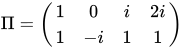
例 2次元複素トーラスの場合、周期行列は次の形式になります。 Π = ( λ 1 、 1 λ 1 、 2 λ 1 、 3 λ 1 、 4 λ 2 、 1 λ 2 、 2 λ 2 、 3 λ 2 、 4 ) {\displaystyle \Pi ={\begin{pmatrix}\lambda _{1,1}&\lambda _{1,2}&\lambda _{1,3}&\lambda _{1,4}\\\lambda _{2,1}&\lambda _{2,2}&\lambda _{2,3}&\lambda _{2,4}\end{pmatrix}}} Π = ( 1 0 私 2 私 1 − 私 1 1 ) {\displaystyle \Pi ={\begin{pmatrix}1&0&i&2i\\1&-i&1&1\end{pmatrix}}}
アーベル多様体の周期行列 射影複素多様体、ひいては代数多様体を与える周期行列を得るには、周期行列がさらにリーマン双線形関係を 満たす必要がある。[ 3 ]
複素多様体の場合X {\displaystyle X} 線束を 関連付ける構成[ 2 ] : L → X {\displaystyle L\to X} π * L → X ~ {\displaystyle \pi ^{*}L\to {\tilde {X}}} 群コホモロジー を用いると自明であるπ 1 ( X ) {\displaystyle \pi _{1}(X)} π * L {\displaystyle \pi ^{*}L} X ~ ≅ C n {\displaystyle {\tilde {X}}\cong \mathbb {C} ^{n}}
自己同型性の因子からの線束 自己同型性の因子が与えられた場合f {\displaystyle f} X {\displaystyle X} X ~ × C → X ~ {\displaystyle {\tilde {X}}\times \mathbb {C} \to {\tilde {X}}} π 1 ( X ) {\displaystyle \pi _{1}(X)} 1 ⋅ ( x 、 t ) = ( 1 ⋅ x 、 f ( 1 、 x ) ⋅ t ) {\displaystyle a\cdot (x,t)=(a\cdot x,f(a,x)\cdot t)} f {\displaystyle f} L = X ~ × C / π 1 ( X ) {\displaystyle L={\tilde {X}}\times \mathbb {C} /\pi _{1}(X)} p : L → X {\displaystyle p:L\to X} π : X ~ → X {\displaystyle \pi :{\tilde {X}}\to X} Z 1 ( π 1 ( X ) 、 H 0 ( O X ~ * ) ) → H 1 ( X 、 O X * ) {\displaystyle Z^{1}(\pi _{1}(X),H^{0}({\mathcal {O}}_{\tilde {X}}^{*}))\to H^{1}(X,{\mathcal {O}}_{X}^{*})} H 1 ( π 1 ( X ) 、 H 0 ( O X ~ * ) ) → カー ( H 1 ( X 、 O X * ) → H 1 ( X ~ 、 O X ~ * ) ) {\displaystyle H^{1}(\pi _{1}(X),H^{0}({\mathcal {O}}_{\tilde {X}}^{*}))\to \ker(H^{1}(X,{\mathcal {O}}_{X}^{*})\to H^{1}({\tilde {X}},{\mathcal {O}}_{\tilde {X}}^{*}))}
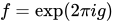
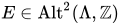
複素トーラス上の線束の第一クラス 指数関数的完全数列 から0 → Z → O X → O X * → 0 {\displaystyle 0\to \mathbb {Z} \to {\mathcal {O}}_{X}\to {\mathcal {O}}_{X}^{*}\to 0} c 1 : H 1 ( O X * ) → H 2 ( X 、 Z ) {\displaystyle c_{1}:H^{1}({\mathcal {O}}_{X}^{*})\to H^{2}(X,\mathbb {Z} )} チャーンクラス 写像です。 の間に同型が存在することがわかります。H 2 ( X 、 Z ) {\displaystyle H^{2}(X,\mathbb {Z} )} Λ {\displaystyle \Lambda } A l t 2 ( Λ 、 Z ) {\displaystyle Alt^{2}(\Lambda ,\mathbb {Z} )} c 1 ( L ) {\displaystyle c_{1}(L)} Z {\displaystyle \mathbb {Z} } E L {\displaystyle E_{L}} Λ {\displaystyle \Lambda } L {\displaystyle L} f = exp ( 2 π 私 g ) {\displaystyle f=\exp(2\pi ig)} E L ( λ 、 μ ) = g ( μ 、 v + λ ) + g ( λ 、 v ) − g ( λ 、 v + μ ) − g ( μ 、 v ) {\displaystyle E_{L}(\lambda ,\mu )=g(\mu ,v+\lambda )+g(\lambda ,v)-g(\lambda ,v+\mu )-g(\mu ,v)} μ 、 λ ∈ Λ {\displaystyle \mu ,\lambda \in \Lambda } v ∈ V {\displaystyle v\in V}
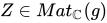
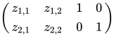
例 正規化された周期行列の場合 Π = ( z 1 、 1 z 1 、 2 1 0 z 2 、 1 z 2 、 2 0 1 ) {\displaystyle \Pi ={\begin{pmatrix}z_{1,1}&z_{1,2}&1&0\\z_{2,1}&z_{2,2}&0&1\end{pmatrix}}} C 2 {\displaystyle \mathbb {C} ^{2}} Λ ⊂ C 2 {\displaystyle \Lambda \subset \mathbb {C} ^{2}} E L {\displaystyle E_{L}} Λ {\displaystyle \Lambda } E L = ( 0 e 2 、 1 e 3 、 1 e 4 、 1 − e 2 、 1 0 e 3 、 2 e 4 、 2 − e 3 、 1 − e 3 、 2 0 e 4 、 3 − e 4 、 1 − e 4 、 2 − e 4 、 3 0 ) {\displaystyle E_{L}={\begin{pmatrix}0&e_{2,1}&e_{3,1}&e_{4,1}\\-e_{2,1}&0&e_{3,2}&e_{4,2}\\-e_{3,1}&-e_{3,2}&0&e_{4,3}\\-e_{4,1}&-e_{4,2}&-e_{4,3}&0\end{pmatrix}}}
交互にZ {\displaystyle \mathbb {Z} } E L {\displaystyle E_{L}} L → X {\displaystyle L\to X} R {\displaystyle \mathbb {R} } R {\displaystyle \mathbb {R} } E : V × V → R {\displaystyle E:V\times V\to \mathbb {R} }
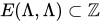
E ( Λ 、 Λ ) ⊆ Z {\displaystyle E(\Lambda ,\Lambda )\subseteq \mathbb {Z} } E ( 私 v 、 私 w ) = E ( v 、 w ) {\displaystyle E(iv,iw)=E(v,w)} v 、 w ∈ V {\displaystyle v,w\in V} これは、ある第一チャーンクラスの拡張である。c 1 ( L ) {\displaystyle c_{1}(L)} L → X {\displaystyle L\to X} H : V × V → C {\displaystyle H:V\times V\to \mathbb {C} }
私は H ( v 、 w ) = E ( v 、 w ) {\displaystyle {\text{Im}}H(v,w)=E(v,w)} H ( v 、 w ) = E ( 私 v 、 w ) + 私 E ( v 、 w ) {\displaystyle H(v,w)=E(iv,w)+iE(v,w)} いかなる場合でもv 、 w ∈ V {\displaystyle v,w\in V}
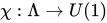
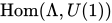
エルミート形式の場合H {\displaystyle H} χ : Λ → U ( 1 ) {\displaystyle \chi :\Lambda \to U(1)} χ ( λ + μ ) = χ ( λ ) χ ( μ ) exp ( 私 π 私は H ( λ 、 μ ) ) {\displaystyle \chi (\lambda +\mu )=\chi (\lambda )\chi (\mu )\exp(i\pi {\text{Im}}H(\lambda ,\mu ))} χ {\displaystyle \chi } キャラクター のように振る舞います。注意:H {\displaystyle H} N S ( X ) {\displaystyle NS(X)} C × X → X {\displaystyle \mathbb {C} \times X\to X} 文字のグループ になります。Λ {\displaystyle \Lambda } 写真 0 ( X ) {\displaystyle {\text{Pic}}^{0}(X)} 0 {\displaystyle 0} X {\displaystyle X} ホーム ( Λ 、 U ( 1 ) ) {\displaystyle {\text{Hom}}(\Lambda ,U(1))} Λ → R → R / Z ≅ U ( 1 ) {\displaystyle \Lambda \to \mathbb {R} \to \mathbb {R} /\mathbb {Z} \cong U(1)} χ ( ⋅ ) = exp ( 2 π 私 v * ( ⋅ ) ) {\displaystyle \chi (\cdot )=\exp \left(2\pi iv^{*}(\cdot )\right)} v * ∈ Λ * {\displaystyle v^{*}\in \Lambda ^{*}} ホーム ( Λ 、 U ( 1 ) ) ≅ R 2 g / Z 2 g {\displaystyle {\text{Hom}}(\Lambda ,U(1))\cong \mathbb {R} ^{2g}/\mathbb {Z} ^{2g}} ( χ 、 H ) {\displaystyle (\chi ,H)} 半文字ペアは グループを形成するP ( Λ ) {\displaystyle {\mathcal {P}}(\Lambda )} ( H 1 、 χ 1 ) * ( H 2 、 χ 2 ) = ( H 1 + H 2 、 χ 1 χ 2 ) {\displaystyle (H_{1},\chi _{1})*(H_{2},\chi _{2})=(H_{1}+H_{2},\chi _{1}\chi _{2})} χ 1 χ 2 {\displaystyle \chi _{1}\chi _{2}} χ 1 χ 2 ( λ + μ ) = χ 1 ( λ + μ ) χ 2 ( λ + μ ) = χ 1 ( λ ) χ 1 ( μ ) χ 2 ( λ ) χ 2 ( μ ) exp ( 私 π 私は H 1 ( λ 、 μ ) ) exp ( 私 π 私は H 2 ( λ 、 μ ) ) = χ 1 χ 2 ( λ ) χ 1 χ 2 ( μ ) exp ( 私 π 私は H 1 ( λ 、 μ ) + 私 π 私は H 2 ( λ 、 μ ) ) {\displaystyle {\begin{aligned}\chi _{1}\chi _{2}(\lambda +\mu )&=\chi _{1}(\lambda +\mu )\chi _{2}(\lambda +\mu )\\&=\chi _{1}(\lambda )\chi _{1}(\mu )\chi _{2}(\lambda )\chi _{2}(\mu )\exp(i\pi {\text{Im}}H_{1}(\lambda ,\mu ))\exp(i\pi {\text{Im}}H_{2}(\lambda ,\mu ))\\&=\chi _{1}\chi _{2}(\lambda )\chi _{1}\chi _{2}(\mu )\exp(i\pi {\text{Im}}H_{1}(\lambda ,\mu )+i\pi {\text{Im}}H_{2}(\lambda ,\mu ))\end{aligned}}} N S ( X ) {\displaystyle NS(X)} ホーム ( Λ 、 U ( 1 ) ) {\displaystyle {\text{Hom}}(\Lambda ,U(1))} 1 → ホーム ( Λ 、 U ( 1 ) ) → P ( Λ ) → N S ( X ) → 1 {\displaystyle 1\to {\text{Hom}}(\Lambda ,U(1))\to {\mathcal {P}}(\Lambda )\to NS(X)\to 1} L ( H 、 χ ) {\displaystyle L(H,\chi )}
半文字ペアと行束 半文字ペアの場合( H 、 χ ) {\displaystyle (H,\chi )} 1 ( H 、 χ ) {\displaystyle a_{(H,\chi )}} Λ {\displaystyle \Lambda } 1 ( H 、 χ ) : Λ × V → C * {\displaystyle a_{(H,\chi )}:\Lambda \times V\to \mathbb {C} ^{*}} 1 ( λ 、 v ) = χ ( λ ) exp ( π H ( v 、 λ ) + π 2 H ( λ 、 λ ) ) {\displaystyle a(\lambda ,v)=\chi (\lambda )\exp(\pi H(v,\lambda )+{\frac {\pi }{2}}H(\lambda ,\lambda ))} 1 ( λ + μ 、 v ) = 1 ( λ 、 v + μ ) 1 ( μ 、 v ) {\displaystyle a(\lambda +\mu ,v)=a(\lambda ,v+\mu )a(\mu ,v)} L ( H 、 χ ) ≅ V × C / Λ {\displaystyle L(H,\chi )\cong V\times \mathbb {C} /\Lambda } Λ {\displaystyle \Lambda } V × C {\displaystyle V\times \mathbb {C} } λ ∘ ( v 、 t ) = ( v + t 、 1 ( H 、 χ ) ( λ 、 v ) t ) {\displaystyle \lambda \circ (v,t)=(v+t,a_{(H,\chi )}(\lambda ,v)t)} L ( H 、 χ ) {\displaystyle L(H,\chi )} 1 ( H 、 χ ) {\displaystyle a_{(H,\chi )}} 自己同型の標準因子 と呼ばれることもあります。L {\displaystyle L} L → X {\displaystyle L\to X} H {\displaystyle H} L {\displaystyle L} P ( Λ ) → 写真 ( X ) {\displaystyle {\mathcal {P}}(\Lambda )\to {\text{Pic}}(X)} 1 → ホーム ( Λ 、 U ( 1 ) ) → P ( Λ ) → N S ( X ) → 0 ↓ ↓ ↓ 1 → 写真 0 ( X ) → 写真 ( X ) → NS ( X ) → 0 {\displaystyle {\begin{matrix}1&\to &{\text{Hom}}(\Lambda ,U(1))&\to &{\mathcal {P}}(\Lambda )&\to &NS(X)&\to 0\\&&\downarrow &&\downarrow &&\downarrow \\1&\to &{\text{Pic}}^{0}(X)&\to &{\text{Pic}}(X)&\to &{\text{NS}}(X)&\to 0\end{matrix}}} アペル=ハンバートの定理 と呼ばれます。
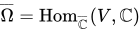
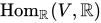
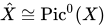
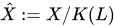
双対複素トーラス 前述のように、格子上の文字は関数として表現できる。 χ ( ⋅ ) = exp ( 2 π 私 v * ( ⋅ ) ) {\displaystyle \chi (\cdot )=\exp \left(2\pi iv^{*}(\cdot )\right)} v ∗ ∈ Λ ∗ {\displaystyle v^{*}\in \Lambda ^{*}} Λ ∗ {\displaystyle \Lambda ^{*}} Ω ¯ = Hom C ¯ ( V , C ) {\displaystyle {\overline {\Omega }}={\text{Hom}}_{\overline {\mathbb {C} }}(V,\mathbb {C} )} antilinear maps, is isomorphic to the real dual vector space Hom R ( V , R ) {\displaystyle {\text{Hom}}_{\mathbb {R} }(V,\mathbb {R} )} Λ ^ = { l ∈ Ω ¯ : ⟨ l , Λ ⟩ ⊆ Z } {\displaystyle {\hat {\Lambda }}=\{l\in {\overline {\Omega }}:\langle l,\Lambda \rangle \subseteq \mathbb {Z} \}} Λ {\displaystyle \Lambda } dual complex torus X ^ ≅ Ω ¯ / Λ ^ {\displaystyle {\hat {X}}\cong {\overline {\Omega }}/{\hat {\Lambda }}} X {\displaystyle X} X ^ ≅ Pic 0 ( X ) {\displaystyle {\hat {X}}\cong {\text{Pic}}^{0}(X)} l {\displaystyle l} l ↦ exp ( 2 π i ⟨ l , ⋅ ⟩ ) {\displaystyle l\mapsto \exp(2\pi i\langle l,\cdot \rangle )} Ω ¯ → Hom ( Λ , U ( 1 ) ) {\displaystyle {\overline {\Omega }}\to {\text{Hom}}(\Lambda ,U(1))} [ 1] : L {\displaystyle L} X {\displaystyle X} K ( L ) {\displaystyle K(L)} X {\displaystyle X} x ∈ X {\displaystyle x\in X} T x ∗ ( L ) ≅ L {\displaystyle T_{x}^{*}(L)\cong L} X ^ := X / K ( L ) {\displaystyle {\hat {X}}:=X/K(L)} X ^ {\displaystyle {\hat {X}}} Pic 0 ( X ) {\displaystyle {\text{Pic}}^{0}(X)}
From the construction of the dual complex torus, it is suggested that there should exist a line bundle P {\displaystyle {\mathcal {P}}} X {\displaystyle X} X {\displaystyle X}
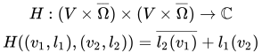
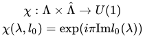
P | X × { [ L ] } ≅ L {\displaystyle {\mathcal {P}}|_{X\times \{[L]\}}\cong L} [ L ] ∈ X ^ {\displaystyle [L]\in {\hat {X}}} L {\displaystyle L} P | { 0 } × X ^ {\displaystyle {\mathcal {P}}|_{\{0\}\times {\hat {X}}}} where the first is the property discussed above, and the second acts as a normalization property. We can construct P {\displaystyle {\mathcal {P}}} H : ( V × Ω ¯ ) × ( V × Ω ¯ ) → C H ( ( v 1 , l 1 ) , ( v 2 , l 2 ) ) = l 2 ( v 1 ) ¯ + l 1 ( v 2 ) {\displaystyle {\begin{matrix}H:(V\times {\overline {\Omega }})\times (V\times {\overline {\Omega }})\to \mathbb {C} \\H((v_{1},l_{1}),(v_{2},l_{2}))={\overline {l_{2}(v_{1})}}+l_{1}(v_{2})\end{matrix}}} χ : Λ × Λ ^ → U ( 1 ) χ ( λ , l 0 ) = exp ( i π Im l 0 ( λ ) ) {\displaystyle {\begin{matrix}\chi :\Lambda \times {\hat {\Lambda }}\to U(1)\\\chi (\lambda ,l_{0})=\exp(i\pi {\text{Im}}l_{0}(\lambda ))\end{matrix}}} H {\displaystyle H} ( H , χ ) {\displaystyle (H,\chi )}
References 1 2 Mumford, David (2008). Abelian varieties . C. P. Ramanujam, I︠U︡. I. Manin. Published for the Tata Institute of Fundamental Research. ISBN 978-8185931869 . OCLC 297809496. 1 2 3 Birkenhake, Christina (2004). Complex Abelian Varieties . Herbert Lange (Second, augmented ed.). Berlin, Heidelberg: Springer Berlin Heidelberg. ISBN 978-3-662-06307-1 OCLC 851380558 ↑ 「リーマン双線形関係」 (PDF) 。 2021年5月31日にオリジナルから アーカイブされました (PDF) 。 ↑ 「楕円曲線の最も単純な場合におけるアペル=ハンバートの定理の働き」 。 Birkenhake, Christina; Lange, Herbert (1999), Complex tori , Progress in Mathematics, vol. 177, Boston, MA: Birkhäuser Boston, ISBN 978-0-8176-4103-0 MR 1713785
複雑な2次元トーラス Ruppert, Wolfgang M. (1990). "アーベル曲面はいつ楕円曲線の積と同型または同種になるのか?" . Mathematische Zeitschrift . 203 : 293–299 . doi : 10.1007/BF02570737 . S2CID 120799085 . マルキージオ、マリーナ・ロザンナ (1998)。「アーベル曲面と楕円曲線の積」。ボッレッティーノ デッロニオーネ マテマティカ イタリアーナ 。1-B (2): 407 – 427。
複雑な隆起部上のゲルベス Ben-Bassat, Oren (2012). "Gerbesと複素トーラスの正則Brauer群". Journal of Noncommutative Geometry . 6 (3): 407–455 . arXiv : 0811.2746 . doi : 10.4171/JNCG/ 96 . S2CID 15049025 . 代替 3 ( Λ 、 Z ) {\displaystyle {\text{Alt}}^{3}(\Lambda ,\mathbb {Z} )} Block, Jonathan; Daenzer, Calder (2008). "接続を持つゲルブの向井双対性". Crelle's Journal arXiv : 0803.1529v2 . ベン・バサット、オーレン (2013)。 「複雑なトーラス上の等変ガーベ」。幾何学と物理学のジャーナル 。64 : 209–221.arXiv : 1102.2312 。 Bibcode : 2013JGP....64..209B。土井 :10.1016/j.geomphys.2012.10.012。S2CID 119599648。 フェルダー、ジョバンニ。エンリケス、アンドレ。ロッシ、カルロ・A.朱、晨昌 (2008)。 「楕円ガンマ関数のガーベ」。デューク数学ジャーナル 。141 . arXiv : math/0601337 。土井 :10.1215/S0012-7094-08-14111-0。S2CID 817920。 









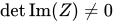


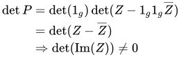
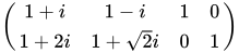











































![{\displaystyle [f]\in H^{1}(\Lambda ,H^{0}(V,{\mathcal {O}}_{V}^{*}))}](https://wikimedia.org/api/rest_v1/media/math/render/svg/d2867b7ac623b81b9c19fa6dfd79b2acfcfbaefc)
![{\displaystyle \phi _{1}[f]=[L]\in {\text{Pic}}(X)}](https://wikimedia.org/api/rest_v1/media/math/render/svg/2912b1b32b2f23e59c14c4370f6c2218cc40276c)




















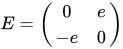


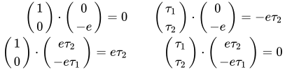





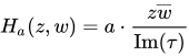

































![{\displaystyle {\mathcal {P}}|_{X\times \{[L]\}}\cong L}](https://wikimedia.org/api/rest_v1/media/math/render/svg/552e41f2b3d9c99df68dcd13abdefa1a35431c39)
![{\displaystyle [L]\in {\hat {X}}}](https://wikimedia.org/api/rest_v1/media/math/render/svg/0b1469e8d8f4615a881557396274ca6e2cc57580)