交点（幾何学）

平行でない2本の直線の交点を決定するために

${\displaystyle a_{1}x+b_{1}y=c_{1},\ a_{2}x+b_{2}y=c_{2}}$

クラメルの公式を用いるか、変数を代入することで、交点の座標が得られる。${\displaystyle (x_{s},y_{s})}$ :

${\displaystyle x_{s}={\frac {c_{1}b_{2}-c_{2}b_{1}}{a_{1}b_{2}-a_{2}b_{1}}},\quad y_{s}={\frac {a_{1}c_{2}-a_{2}c_{1}}{a_{1}b_{2}-a_{2}b_{1}}}.\ }$

（もし${\displaystyle a_{1}b_{2}-a_{2}b_{1}=0}$線は平行であり、これらの式はゼロ除算を含むため使用できません。

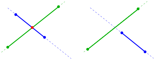
平行でない2つの線分の場合${\displaystyle (x_{1},y_{1}),(x_{2},y_{2})}$そして${\displaystyle (x_{3},y_{3}),(x_{4},y_{4})}$必ずしも交点が存在するとは限らない（図を参照）。なぜなら交点が${\displaystyle (x_{0},y_{0})}$対応する線分は、線分内に含まれる必要はありません。この状況を確認するために、線分のパラメトリック表現を使用します。

${\displaystyle (x(s),y(s))=(x_{1}+s(x_{2}-x_{1}),y_{1}+s(y_{2}-y_{1})),}$

${\displaystyle (x(t),y(t))=(x_{3}+t(x_{4}-x_{3}),y_{3}+t(y_{4}-y_{3})).}$

線分は一点でのみ交わる。${\displaystyle (x_{0},y_{0})}$対応するパラメータが${\displaystyle s_{0},t_{0}}$条件を満たす${\displaystyle 0\leq s_{0},t_{0}\leq 1}$パラメータ${\displaystyle s_{0},t_{0}}$線形システムの解

${\displaystyle s(x_{2}-x_{1})-t(x_{4}-x_{3})=x_{3}-x_{1},}$

${\displaystyle s(y_{2}-y_{1})-t(y_{4}-y_{3})=y_{3}-y_{1}\ .}$

sとtについては、クラメルの公式（上記参照）を用いて解くことができます。条件が${\displaystyle 0\leq s_{0},t_{0}\leq 1}$1つの挿入が満たされる${\displaystyle s_{0}}$または${\displaystyle t_{0}}$対応するパラメトリック表現に変換し、交点を取得する${\displaystyle (x_{0},y_{0})}$。

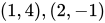
例: 線分の場合${\displaystyle (1,1),(3,2)}$そして${\displaystyle (1,4),(2,-1)}$線形システムが得られる

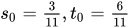
${\displaystyle 2s-t=0}$

${\displaystyle s+5t=3}$

そして${\displaystyle s_{0}={\tfrac {3}{11}},t_{0}={\tfrac {6}{11}}}$つまり、線は点で交差する。${\displaystyle ({\tfrac {17}{11}},{\tfrac {14}{11}})}$。

注記：点のペアによって決定される線分ではなく直線を考慮すると、各条件は${\displaystyle 0\leq s_{0},t_{0}\leq 1}$削除することができ、この方法では線の交点が得られます（上記を参照）。

交差点については

• ライン${\displaystyle ax+by=c}$そして円${\displaystyle x^{2}+y^{2}=r^{2}}$

直線の方程式をxまたはyについて解き、それを円の方程式に代入すると、（二次方程式の公式を用いて）解が得られます。${\displaystyle (x_{1},y_{1}),(x_{2},y_{2})}$と

${\displaystyle x_{1/2}={\frac {ac\pm b{\sqrt {r^{2}(a^{2}+b^{2})-c^{2}}}}{a^{2}+b^{2}}}\ ,}$

${\displaystyle y_{1/2}={\frac {bc\mp a{\sqrt {r^{2}(a^{2}+b^{2})-c^{2}}}}{a^{2}+b^{2}}}\ ,}$

もし${\displaystyle r^{2}(a^{2}+b^{2})-c^{2}>0\ .}$この条件が厳密な不等式で成り立つ場合、交点は2つ存在する。この場合、その直線は円の割線と呼ばれ、交点を結ぶ線分は円の弦と呼ばれる。

もし${\displaystyle r^{2}(a^{2}+b^{2})-c^{2}=0}$不等式が成り立つ場合、交点はただ一つであり、直線は円に接する。不等式が成り立たない場合、直線は円と交わらない。

交点を素早く求めるもう1つの方法は、アンザッツです。${\displaystyle (x_{1/2},y_{1/2})=s(a,b)\pm t(b,-a)}$まず、${\displaystyle s}$直線の方程式を用いると、それは次のように簡略化される。${\displaystyle s(a^{2}+b^{2})=c}$そして、${\displaystyle t}$円の方程式を用いると、それは次のように簡略化される。${\displaystyle (s^{2}+t^{2})(a^{2}+b^{2})=r^{2}}$。

円の中点が原点でない場合は、^{[ 1 ]}を参照してください。直線と放物線または双曲線の交点も同様に扱うことができます。

2つの円の交点の決定

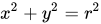
• ${\displaystyle (x-x_{1})^{2}+(y-y_{1})^{2}=r_{1}^{2},\ \quad (x-x_{2})^{2}+(y-y_{2})^{2}=r_{2}^{2}}$

これは、直線と円の交点を求めるという前述のケースに帰着します。与えられた2つの方程式を引き算すると、直線の方程式が得られます。

${\displaystyle 2(x_{2}-x_{1})x+2(y_{2}-y_{1})y=r_{1}^{2}-x_{1}^{2}-y_{1}^{2}-r_{2}^{2}+x_{2}^{2}+y_{2}^{2}.}$

この特別な線は、2つの円の根号線です。

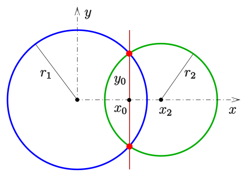
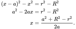
特別なケース${\displaystyle \;x_{1}=y_{1}=y_{2}=0}$ この場合、 原点は最初の円の中心であり、2番目の中心はx軸上にあります（図参照）。根号線の式は次のように簡略化されます。${\displaystyle \;2x_{2}x=r_{1}^{2}-r_{2}^{2}+x_{2}^{2}\;}$交点は次のように表すことができます。${\displaystyle (x_{0},\pm y_{0})}$と

${\displaystyle x_{0}={\frac {r_{1}^{2}-r_{2}^{2}+x_{2}^{2}}{2x_{2}}},\quad y_{0}={\sqrt {r_{1}^{2}-x_{0}^{2}}}\ .}$

の場合${\displaystyle r_{1}^{2}<x_{0}^{2}}$ これらの円には共通点がありません。${\displaystyle r_{1}^{2}=x_{0}^{2}}$これらの円は共通点を1つ持ち、根号線は共通の接線である。

上記のような一般的なケースは、シフトと回転によって特殊なケースに変換することができる。

2つの円盤（2つの円の内部）の交わりによって、レンズと呼ばれる形状が形成されます。

The problem of intersection of an ellipse/hyperbola/parabola with another conic section leads to a system of quadratic equations, which can be solved in special cases easily by elimination of one coordinate. Special properties of conic sections may be used to obtain a solution. In general the intersection points can be determined by solving the equation by a Newton iteration. If a) both conics are given implicitly (by an equation) a 2-dimensional Newton iteration b) one implicitly and the other parametrically given a 1-dimensional Newton iteration is necessary. See next section.

Two curves in ${\displaystyle \mathbb {R} ^{2}}$ (two-dimensional space), which are continuously differentiable (i.e. there is no sharp bend), have an intersection point, if they have a point of the plane in common and have at this point (see diagram):

a) different tangent lines (transversal intersection, after transversality), or

b) the tangent line in common and they are crossing each other (touching intersection, after tangency).

If both the curves have a point S and the tangent line there in common but do not cross each other, they are just touching at point S.

Because touching intersections appear rarely and are difficult to deal with, the following considerations omit this case. In any case below all necessary differential conditions are presupposed. The determination of intersection points always leads to one or two non-linear equations which can be solved by Newton iteration. A list of the appearing cases follows:

• If both curves are explicitly given: ${\displaystyle y=f_{1}(x),\ y=f_{2}(x)}$, equating them yields the equation

${\displaystyle f_{1}(x)=f_{2}(x)\ .}$

• If both curves are parametrically given: ${\displaystyle C_{1}:(x_{1}(t),y_{1}(t)),\ C_{2}:(x_{2}(s),y_{2}(s)).}$

Equating them yields two equations in two variables:

${\displaystyle x_{1}(t)=x_{2}(s),\ y_{1}(t)=y_{2}(s)\ .}$

• If one curve is parametrically and the other implicitly given: ${\displaystyle C_{1}:(x_{1}(t),y_{1}(t)),\ C_{2}:f(x,y)=0.}$

This is the simplest case besides the explicit case. One has to insert the parametric representation of ${\displaystyle C_{1}}$ into the equation ${\displaystyle f(x,y)=0}$ of curve ${\displaystyle C_{2}}$ and one gets the equation:

${\displaystyle f(x_{1}(t),y_{2}(t))=0\ .}$

• If both curves are implicitly given: ${\displaystyle C_{1}:f_{1}(x,y)=0,\ C_{2}:f_{2}(x,y)=0.}$

Here, an intersection point is a solution of the system

${\displaystyle f_{1}(x,y)=0,\ f_{2}(x,y)=0\ .}$

ニュートン法の反復には、曲線を視覚化することで得られる便利な初期値が必要です。パラメトリックまたは明示的に与えられた曲線は、任意のパラメータtまたはxに対して対応する点を簡単に計算できるため、簡単に視覚化できます。暗黙的に与えられた曲線の場合、この作業はそれほど簡単ではありません。この場合、初期値と反復を使用して曲線上の点を決定する必要があります。^{[ 2 ]を参照してください。}

例：

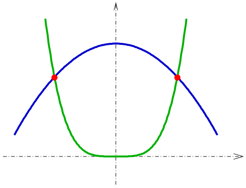
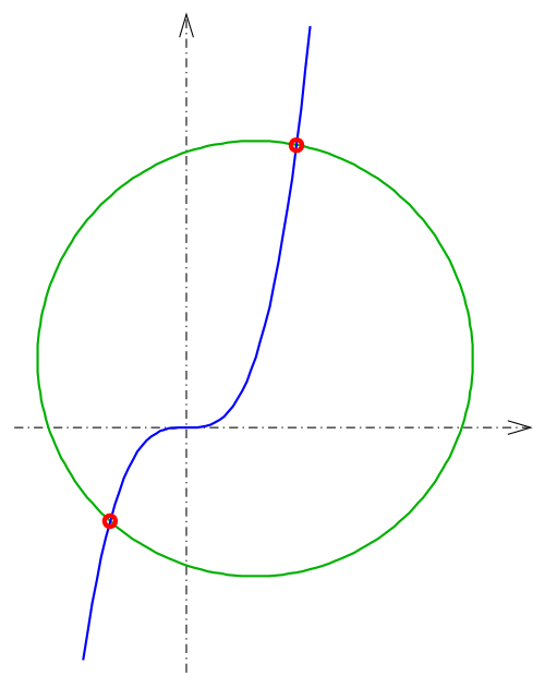
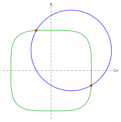
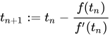
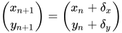
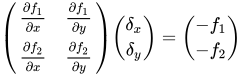
1:${\displaystyle C_{1}:(t,t^{3})}$そして円${\displaystyle C_{2}:(x-1)^{2}+(y-1)^{2}-10=0}$（図を参照）。

ニュートン反復法${\displaystyle t_{n+1}:=t_{n}-{\frac {f(t_{n})}{f'(t_{n})}}}$関数

${\displaystyle f(t)=(t-1)^{2}+(t^{3}-1)^{2}-10}$実行する必要があります。開始値としては、-1と1.5を選択できます。

交点は次のとおりです: (−1.1073, −1.3578)、(1.6011, 4.1046)

2:${\displaystyle C_{1}:f_{1}(x,y)=x^{4}+y^{4}-1=0,}$

${\displaystyle C_{2}:f_{2}(x,y)=(x-0.5)^{2}+(y-0.5)^{2}-1=0}$（図を参照）。

ニュートン反復法

${\displaystyle {x_{n+1} \choose y_{n+1}}={x_{n}+\delta _{x} \choose y_{n}+\delta _{y}}}$実行する必要がある場所${\displaystyle {\delta _{x} \choose \delta _{y}}}$線形システムの解は

${\displaystyle {\begin{pmatrix}{\frac {\partial f_{1}}{\partial x}}&{\frac {\partial f_{1}}{\partial y}}\\{\frac {\partial f_{2}}{\partial x}}&{\frac {\partial f_{2}}{\partial y}}\end{pmatrix}}{\delta _{x} \choose \delta _{y}}={-f_{1} \choose -f_{2}}}$地点で${\displaystyle (x_{n},y_{n})}$開始値としては、（−0.5, 1）と（1, −0.5）を選択できます。

この線形方程式系は、クラメルの公式を用いて解くことができる。

交点は（−0.3686, 0.9953）と（0.9953, −0.3686）です。

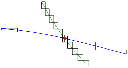
2 つの多角形の交点を決定したい場合は、多角形の任意の線分のペアの交点をチェックできます (上記参照)。セグメントが多い多角形の場合、この方法はかなり時間がかかります。実際には、ウィンドウ テストを使用して交点アルゴリズムを高速化します。この場合、多角形を小さなサブ多角形に分割し、任意のサブ多角形に対して最小のウィンドウ (座標軸に平行な辺を持つ長方形) を決定します。2 つの線分の交点の時間のかかる決定を開始する前に、任意のウィンドウのペアに共通点があるかどうかをテストします。参照。^{[ 3 ]}

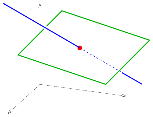
3次元空間において、直線と平面が一般の位置関係で交わる点は点である。

一般的に、空間内の線はパラメトリックに表現される。 ${\displaystyle (x(t),y(t),z(t))}$そして方程式による平面${\displaystyle ax+by+cz=d}$パラメータ表現を方程式に代入すると、線形方程式が得られる。

${\displaystyle ax(t)+by(t)+cz(t)=d\ ,}$

パラメータの場合${\displaystyle t_{0}}$交点の${\displaystyle (x(t_{0}),y(t_{0}),z(t_{0}))}$。

線形方程式に解がない場合、その直線は平面上にあるか、平面に平行である。

直線が2つの交差する平面によって定義される場合${\displaystyle \varepsilon _{i}:\ {\vec {n}}_{i}\cdot {\vec {x}}=d_{i},\ i=1,2}$そして、第三の平面と交差するべきである${\displaystyle \varepsilon _{3}:\ {\vec {n}}_{3}\cdot {\vec {x}}=d_{3}}$そのため、3つの平面の共通交点を評価する必要がある。

3機の飛行機${\displaystyle \varepsilon _{i}:\ {\vec {n}}_{i}\cdot {\vec {x}}=d_{i},\ i=1,2,3}$線形独立な法線ベクトルを持つ${\displaystyle {\vec {n}}_{1},{\vec {n}}_{2},{\vec {n}}_{3}}$交点を持つ

${\displaystyle {\vec {p}}_{0}={\frac {d_{1}({\vec {n}}_{2}\times {\vec {n}}_{3})+d_{2}({\vec {n}}_{3}\times {\vec {n}}_{1})+d_{3}({\vec {n}}_{1}\times {\vec {n}}_{2})}{{\vec {n}}_{1}\cdot ({\vec {n}}_{2}\times {\vec {n}}_{3})}}\ .}$

証明のためには、${\displaystyle {\vec {n}}_{i}\cdot {\vec {p}}_{0}=d_{i},\ i=1,2,3,}$スカラー三重積の規則を使用します。スカラー三重積が 0 に等しい場合、平面は三重交点を持たないか、直線になります (または、3 つの平面がすべて同じ場合は平面になります)。

平面の場合と同様に、以下のケースでは非線形システムが生じ、1次元または3次元のニュートン反復法を用いて解くことができる。^{[ 4 ]}

• パラメトリック曲線${\displaystyle C:(x(t),y(t),z(t))}$そして

パラメトリック曲面${\displaystyle S:(x(u,v),y(u,v),z(u,v))\ ,}$

• パラメトリック曲線${\displaystyle C:(x(t),y(t),z(t))}$そして

暗黙の表面${\displaystyle S:f(x,y,z)=0\ .}$

例：

パラメトリック曲線${\displaystyle C:(t,t^{2},t^{3})}$ そして

暗黙の表面${\displaystyle S:x^{4}+y^{4}+z^{4}-1=0}$（写真参照）

交点は (−0.8587, 0.7374, −0.6332)、(0.8587, 0.7374, 0.6332) です。

直線と球の交点は、単純な特殊なケースである。

直線と平面の場合と同様に、曲線と曲面の交点は、一般的な位置では離散的な点から構成されるが、曲線は曲面内に部分的に、あるいは完全に含まれる場合がある。

2つの曲面が交差すると、交曲線ができます。最も単純な例は、平行でない2つの平面の交線です。

球と平面の交点が空集合または一点でない場合、それは円になります。これは次のように説明できます。

S を中心Oの球、PをSと交わる平面とする。OEをPに垂直に引き、Pとの交点をEとする。交点内の任意の 2 つの異なる点をAとBとする。すると、 AOEとBOE は共通の辺OEを持ち、斜辺AOとBO が等しい直角三角形となる。したがって、残りの辺AEとBEも等しい。これにより、交点内のすべての点が平面P内の点Eから同じ距離にあることが証明される。言い換えれば、交点内のすべての点は中心Eの円C上にある。^{[ 5 ]}これにより、 PとSの交点がCに含まれることが証明される。OE は円の軸であることに注意する。

ここで、円Cの点Dを考えます。CはP内にあるので、Dも P 内にあります。一方、三角形AOEとDOE は、共通の辺OEを持ち、2辺EAとEDが等しい直角三角形です。したがって、斜辺AOとDO は等しく、 Sの半径に等しいので、D はS内にあります。これにより、C はPとSの交点に含まれることが証明されます。

その結果として、球面上には、与えられた3点を通る円がちょうど1つだけ存在する。^{[ 6 ]}

この証明は、円上の点がすべてその極のいずれかから共通の角度距離にあることを示すように拡張できる。 ^{[ 7 ]}

円錐曲線も比較してみてください。円錐曲線は楕円を生成することができます。

2 つの球の非自明な交差が円であることを示すために、(一般性を失うことなく) 1 つの球 (半径 ) が${\displaystyle R}$) は原点を中心とする。この球面上の点が次の条件を満たす。

${\displaystyle x^{2}+y^{2}+z^{2}=R^{2}.}$

また、一般性を失うことなく、半径が の 2 番目の球を仮定する。${\displaystyle r}$は、正のx軸上の距離にある点を中心としています。${\displaystyle a}$原点から。その点は

${\displaystyle (x-a)^{2}+y^{2}+z^{2}=r^{2}.}$

球の交点は、両方の式を満たす点の集合です。式を引き算すると、

${\displaystyle {\begin{aligned}(x-a)^{2}-x^{2}&=r^{2}-R^{2}\\a^{2}-2ax&=r^{2}-R^{2}\\x&={\frac {a^{2}+R^{2}-r^{2}}{2a}}.\end{aligned}}}$

特異なケース${\displaystyle a=0}$球体は同心円状です。可能性は2つあります。${\displaystyle R=r}$球が一致し、交差部分が球全体である場合、${\displaystyle R\not =r}$の場合、球は互いに分離しており、交差部分は空である。a がゼロでない場合、交差部分は、この x 座標を持つ垂直平面上にあり、その平面は両方の球と交差するか、両方の球に接するか、または両方の球の外側にある可能性がある。この結果は、球と平面の交差に関する以前の証明から導かれる。