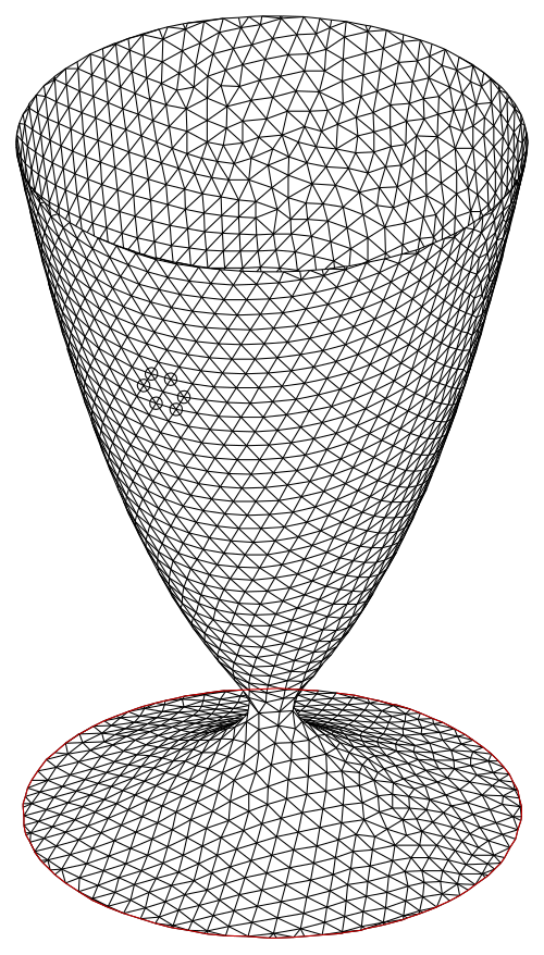
暗黙の表面トーラス(R = 40、a = 15) 。 種数2の暗黙的な曲面。 暗黙の非代数曲面(ワイングラス )。 数学 において、陰関数曲面とは、 ユークリッド空間 において方程式によって定義される曲面のこと である。
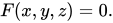
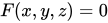
F ( x 、 y 、 z ) = 0. {\displaystyle F(x,y,z)=0.} 陰関数曲面 とは、 3つの変数を持つ関数 の零点 の集合のことです。陰関数と x 、y 、z について解かれていないことを意味します。
関数のグラフは通常、方程式で表されます。z = f ( x 、 y ) {\displaystyle z=f(x,y)} これは明示的 表現と呼ばれます。曲面の3つ目の重要な記述は、パラメトリック ( x ( s 、 t ) 、 y ( s 、 t ) 、 z ( s 、 t ) ) {\displaystyle (x(s,t),y(s,t),z(s,t))} x 、y 、z座標は 3 つの関数で表されます。 x ( s 、 t ) 、 y ( s 、 t ) 、 z ( s 、 t ) {\displaystyle x(s,t)\,,y(s,t)\,,z(s,t)} s 、 t {\displaystyle s,t} z = f ( x 、 y ) {\displaystyle z=f(x,y)} z − f ( x 、 y ) = 0 {\displaystyle zf(x,y)=0} ( s 、 t 、 f ( s 、 t ) ) {\displaystyle (s,t,f(s,t))}
例 :
飛行機 x + 2 y − 3 z + 1 = 0. {\displaystyle x+2y-3z+1=0.} 球体 x 2 + y 2 + z 2 − 4 = 0. {\displaystyle x^{2}+y^{2}+z^{2}-4=0.} トーラス ( x 2 + y 2 + z 2 + R 2 − 1 2 ) 2 − 4 R 2 ( x 2 + y 2 ) = 0. {\displaystyle (x^{2}+y^{2}+z^{2}+R^{2}-a^{2})^{2}-4R^{2}(x^{2}+y^{2})=0.} 種数 2の表面:2 y ( y 2 − 3 x 2 ) ( 1 − z 2 ) + ( x 2 + y 2 ) 2 − ( 9 z 2 − 1 ) ( 1 − z 2 ) = 0 {\displaystyle 2y(y^{2}-3x^{2})(1-z^{2})+(x^{2}+y^{2})^{2}-(9z^{2}-1)(1-z^{2})=0} 革命の 表面x 2 + y 2 − ( ln ( z + 3.2 ) ) 2 − 0.02 = 0 {\displaystyle x^{2}+y^{2}-(\ln(z+3.2))^{2}-0.02=0} 「ワイングラス 」を参照)。平面、球、トーラスについては、単純な媒介変数表示が存在する。しかし、4番目の例ではそうではない。
陰関数定理は、 方程式が成り立つ条件を記述する。F ( x 、 y 、 z ) = 0 {\displaystyle F(x,y,z)=0} x 、y 、z については(少なくとも暗黙的に)解くことができます。しかし一般に、解を明示的に示すことはできません。この定理は、接平面 、曲面法線 、曲率 (下記参照)など、曲面の基本的な幾何学的特徴を計算する鍵となります。しかし、重要な欠点があります。それは、視覚化が難しいことです。
もしF ( x 、 y 、 z ) {\displaystyle F(x,y,z)} x 、y 、z に関する多項式である場合、その曲面は代数的で あると呼ばれます。例 5 は非 代数的です。
視覚化の難しさにもかかわらず、暗黙曲面は、理論的(例えばシュタイナー曲面 )にも実際的(下記参照)にも興味深い曲面を生成するための比較的単純な手法を提供する。
以下の考察全体を通して、陰関数曲面は方程式で表される。 F ( x 、 y 、 z ) = 0 {\displaystyle F(x,y,z)=0} F {\displaystyle F} 微分可能性 の 必要条件を満たす。F {\displaystyle F} F x 、 F y 、 F z 、 F x x 、 … {\displaystyle F_{x},F_{y},F_{z},F_{xx},\ldots }
接平面と法線ベクトル 表面点( x 0 、 y 0 、 z 0 ) {\displaystyle (x_{0},y_{0},z_{0})} は 、勾配が F {\displaystyle F} ( x 0 、 y 0 、 z 0 ) {\displaystyle (x_{0},y_{0},z_{0})} ( 0 、 0 、 0 ) {\displaystyle (0,0,0)}
( F x ( x 0 、 y 0 、 z 0 ) 、 F y ( x 0 、 y 0 、 z 0 ) 、 F z ( x 0 、 y 0 、 z 0 ) ) ≠ ( 0 、 0 、 0 ) {\displaystyle (F_{x}(x_{0},y_{0},z_{0}),F_{y}(x_{0},y_{0},z_{0}),F_{z}(x_{0},y_{0},z_{0}))\neq (0,0,0)} 表面の点( x 0 、 y 0 、 z 0 ) {\displaystyle (x_{0},y_{0},z_{0})} ではなく、 単数形 と呼ばれます。
正則点における接平面の方程式( x 0 、 y 0 、 z 0 ) {\displaystyle (x_{0},y_{0},z_{0})}
F x ( x 0 、 y 0 、 z 0 ) ( x − x 0 ) + F y ( x 0 、 y 0 、 z 0 ) ( y − y 0 ) + F z ( x 0 、 y 0 、 z 0 ) ( z − z 0 ) = 0 、 {\displaystyle F_{x}(x_{0},y_{0},z_{0})(x-x_{0})+F_{y}(x_{0},y_{0},z_{0})(y-y_{0})+F_{z}(x_{0},y_{0},z_{0})(z-z_{0})=0,} 法線ベクトル は
n ( x 0 、 y 0 、 z 0 ) = ( F x ( x 0 、 y 0 、 z 0 ) 、 F y ( x 0 、 y 0 、 z 0 ) 、 F z ( x 0 、 y 0 、 z 0 ) ) T 。 {\displaystyle \mathbf {n} (x_{0},y_{0},z_{0})=(F_{x}(x_{0},y_{0},z_{0}),F_{y}(x_{0},y_{0},z_{0}),F_{z}(x_{0},y_{0},z_{0}))^{T}.}
通常の曲率 式をシンプルに保つために引数は( x 0 、 y 0 、 z 0 ) {\displaystyle (x_{0},y_{0},z_{0})}
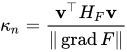
κ n = v ⊤ H F v ‖ 卒業生 F ‖ {\displaystyle \kappa _{n}={\frac {\mathbf {v} ^{\top }H_{F}\mathbf {v} }{\|\operatorname {grad} F\|}}} は、単位接線方向における正則点における曲面の法線曲率である。v {\displaystyle \mathbf {v} } H F {\displaystyle H_{F}} はヘッセ 行列ですF {\displaystyle F}
この公式の証明は、(陰関数曲線の場合と同様に)陰関数定理とパラメトリック曲面 の法線曲率の公式に基づいています。
陰関数曲面の応用 陰関数曲線の場合と同様に、単純な基本要素に代数演算(加算、乗算)を適用することで、目的の形状を持つ陰関数曲面を生成するのは容易な作業です。
4つの点電荷の等電位面
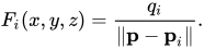
点電荷の等電位面 点電荷の電位 q 私 {\displaystyle q_{i}} p 私 = ( x 私 、 y 私 、 z 私 ) {\displaystyle \mathbf {p} _{i}=(x_{i},y_{i},z_{i})} p = ( x 、 y 、 z ) {\displaystyle \mathbf {p} =(x,y,z)}
F 私 ( x 、 y 、 z ) = q 私 ‖ p − p 私 ‖ 。 {\displaystyle F_{i}(x,y,z)={\frac {q_{i}}{\|\mathbf {p} -\mathbf {p} _{i}\|}}.} 電位値の等電位面c {\displaystyle c} F 私 ( x 、 y 、 z ) − c = 0 {\displaystyle F_{i}(x,y,z)-c=0} p 私 {\displaystyle \mathbf {p} _{i}}
潜在力4 {\displaystyle 4}
F ( x 、 y 、 z ) = q 1 ‖ p − p 1 ‖ + q 2 ‖ p − p 2 ‖ + q 3 ‖ p − p 3 ‖ + q 4 ‖ p − p 4 ‖ 。 {\displaystyle F(x,y,z)={\frac {q_{1}}{\|\mathbf {p} -\mathbf {p} _{1}\|}}+{\frac {q_{2}}{\|\mathbf {p} -\mathbf {p} _{2}\|}}+{\frac {q_{3}}{\|\mathbf {p} -\mathbf {p} _{3}\|}}+{\frac {q_{4}}{\|\mathbf {p} -\mathbf {p} _{4}\|}}.} 図では、4つの電荷は1に等しく、以下の点に位置しています。 ( ± 1 、 ± 1 、 0 ) {\displaystyle (\pm 1,\pm 1,0)} F ( x 、 y 、 z ) − 2.8 = 0 {\displaystyle F(x,y,z)-2.8=0}
一定距離製品表面 カッシーニの楕円は、与えられた2点までの距離の積が一定となる点の集合として定義できる(対照的に、楕円の場合は距離の和 が一定となる)。同様に、陰関数曲面は、複数の固定点までの距離の積が一定となることで定義できる。
図の変形 において、左上の表面はこの規則によって生成されます。
F ( x 、 y 、 z ) = ( x − 1 ) 2 + y 2 + z 2 ⋅ ( x + 1 ) 2 + y 2 + z 2 ⋅ x 2 + ( y − 1 ) 2 + z 2 ⋅ x 2 + ( y + 1 ) 2 + z 2 {\displaystyle {\begin{aligned}F(x,y,z)={}&{\sqrt {(x-1)^{2}+y^{2}+z^{2}}}\cdot {\sqrt {(x+1)^{2}+y^{2}+z^{2}}}\\&\quad \cdot {\sqrt {x^{2}+(y-1)^{2}+z^{2}}}\cdot {\sqrt {x^{2}+(y+1)^{2}+z^{2}}}\end{aligned}}} 一定距離積面 F ( x 、 y 、 z ) − 1.1 = 0 {\displaystyle F(x,y,z)-1.1=0}
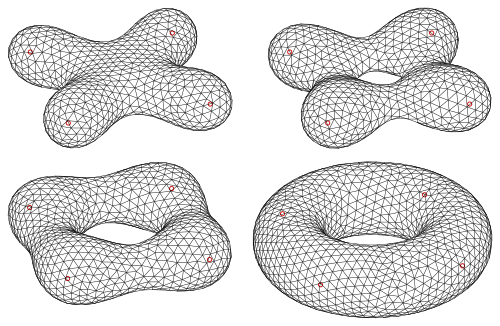
2つの暗黙の曲面間の変形:トーラスと定距離積曲面。
新しい陰関数曲面を生成するもう一つの簡単な方法は、陰関数曲面の変形 またはホモトピー
2つの陰関数曲面の場合F 0 ( x 、 y 、 z ) = 0 、 F 1 ( x 、 y 、 z ) = 0 {\displaystyle F_{0}(x,y,z)=0,F_{1}(x,y,z)=0} μ ∈ [ 0 、 1 ] {\displaystyle \mu \in [0,1]}
F μ ( x 、 y 、 z ) = μ F 1 ( x 、 y 、 z ) + ( 1 − μ ) F 0 ( x 、 y 、 z ) = 0 {\displaystyle F_{\mu }(x,y,z)=\mu F_{1}(x,y,z)+(1-\mu )\,F_{0}(x,y,z)=0} 図では、設計パラメータは順次μ = 0 、 0.33 、 0.66 、 1 {\displaystyle \mu =0,\,0.33,\,0.66,\,1}
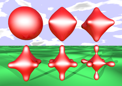
3つのトーラスの近似(平行投影 ) POV-Ray画像(中心投影)。
いくつかの陰関数曲面の滑らかな近似 Π {\displaystyle \Pi } [ 1] R 3 {\displaystyle R^{3}} f i ∈ R [ x 1 , … , x n ] ( i = 1 , … , k ) {\displaystyle f_{i}\in \mathbb {R} [x_{1},\ldots ,x_{n}](i=1,\ldots ,k)}
F ( x , y , z ) = ∏ i f i ( x , y , z ) − r {\displaystyle F(x,y,z)=\prod _{i}f_{i}(x,y,z)-r} [ 1] where r ∈ R {\displaystyle r\in \mathbb {R} }
Analogously to the smooth approximation with implicit curves, the equation
F ( x , y , z ) = F 1 ( x , y , z ) ⋅ F 2 ( x , y , z ) ⋅ F 3 ( x , y , z ) − r = 0 {\displaystyle F(x,y,z)=F_{1}(x,y,z)\cdot F_{2}(x,y,z)\cdot F_{3}(x,y,z)-r=0} represents for suitable parameters c {\displaystyle c}
F 1 = ( x 2 + y 2 + z 2 + R 2 − a 2 ) 2 − 4 R 2 ( x 2 + y 2 ) = 0 , F 2 = ( x 2 + y 2 + z 2 + R 2 − a 2 ) 2 − 4 R 2 ( x 2 + z 2 ) = 0 , F 3 = ( x 2 + y 2 + z 2 + R 2 − a 2 ) 2 − 4 R 2 ( y 2 + z 2 ) = 0. {\displaystyle {\begin{aligned}F_{1}=(x^{2}+y^{2}+z^{2}+R^{2}-a^{2})^{2}-4R^{2}(x^{2}+y^{2})=0,\\[3pt]F_{2}=(x^{2}+y^{2}+z^{2}+R^{2}-a^{2})^{2}-4R^{2}(x^{2}+z^{2})=0,\\[3pt]F_{3}=(x^{2}+y^{2}+z^{2}+R^{2}-a^{2})^{2}-4R^{2}(y^{2}+z^{2})=0.\end{aligned}}} (In the diagram the parameters are R = 1 , a = 0.2 , r = 0.01. {\displaystyle R=1,\,a=0.2,\,r=0.01.}
POV-Ray image: metamorphoses between a sphere and a constant distance product surface (6 points).
Visualization of implicit surfaces There are various algorithms for rendering implicit surfaces,[ 2] marching cubes algorithm .[ 3] surface triangulation ) and the second relies on ray tracing which determines intersection points of rays with the surface.[ 4] sphere tracing , using a signed distance function to find the distance to the surface.[ 5]
Implicit surface software
Free implicit surface software Open-source or free software supporting algebraic implicit surface modelling:
K3DSurf— A program to visualize and manipulate Mathematical models in 3-6 dimensions. K3DSurf supports Parametric equations and Isosurfaces CGAL PyVista [ 6] VTK for easier handling of implicit surfaces. Simplified API for rendering and manipulating implicit surfaces. It can integrate with numpy .Some Blender SculptsFEM ImpliSolid[ 7] Houdini [ 8 ] POV-Ray [ 9 ] 視覚ベースの表面再構成では、表面の統計的モデリングに暗黙関数を使用します。SDFStudio、[ 10 ] [ 11 ] [ 12 ] マーチングキューブ法 や一般的な画像ベースのメッシュ生成の 文脈において、陰関数曲面の多角形化のための様々なソフトウェアが存在するが、それらは必ずしも代数的な閉形式体に基づいているわけではない。
暗黙の表面ソフトウェアを使用する産業用または商用ソフトウェア
参考文献 1 2 Adriano N. Raposo; Abel JP Gomes (2019). "Pi-surfaces: 3D オブジェクトの構成的合成に向けた暗黙の曲面の積". WSCG 2019 27. 中央ヨーロッパにおけるコンピュータグラフィックス、可視化、コンピュータビジョンに関する国際会議. arXiv : 1906.06751 . ↑ Jules Bloomenthal; Chandrajit Bajaj; Brian Wyvill (1997年8月15日). Introduction to Implicit Surfaces . Morgan Kaufmann. ISBN 978-1-55860-233-5 。↑ イアン・スティーブンソン(2004年12月1日)。 プロダクションレンダリング:設計と実装 。シュプリンガー・サイエンス&ビジネス・メディア 。ISBN 978-1-85233-821-3 。↑ エリック・ヘインズ、トーマス・アケニン=モラー:レイ・トレーシング・ジェムズ 、シュプリンガー、2019年、 ISBN 978-1-4842-4427-2 ↑ Hardy, Alexandre; Steeb, Willi-Hans (2008). Mathematical Tools in Computer Graphics with C# Implementations . World Scientific. ISBN 978-981-279-102-3 。↑ PyVista: https://github.com/pyvista/pyvista/blob/main/LICENSE ↑ インプリソリッド ↑ cgwiki: ボリューム: Houdini & CG のヒント: https://tokeru.com/cgwiki/HoudiniVolumes.html (2025年1月20日アクセス) ↑ https://www.povray.org/documentation/view/3.7.0/301/ ↑ SDFStudio ↑ ジオ・ニューズ ↑ PointSDF ↑ アルテアにおける暗黙的モデリングを用いた(確率的)格子設計(パトリック・J・フリン著) ↑ Welch, Ken. 「Altair Inspire 2023: ... Implicit Modeling Solution」Altair Blog、2023年11月30日。入手先:2025年1月20日アクセス。
さらに読む Gomes, A.、Voiculescu, I.、Jorge, J.、Wyvill, B.、Galbraith, C.:暗黙の曲線と曲面: 数学、データ構造、アルゴリズム 、2009 年、Springer-Verlag London、ISBN 978-1-84882-405-8 Thorpe:微分幾何学の基礎的トピック 、Springer-Verlag、ニューヨーク、1979年、ISBN 0-387-90357-7







































![{\displaystyle \mu \in [0,1]}](https://wikimedia.org/api/rest_v1/media/math/render/svg/030ca0eebf53f89d13f475805d065c80355c9390)




}](https://wikimedia.org/api/rest_v1/media/math/render/svg/b9d28099267fd6eb0853dc52433279c27d65043f)



![{\displaystyle {\begin{aligned}F_{1}=(x^{2}+y^{2}+z^{2}+R^{2}-a^{2})^{2}-4R^{2}(x^{2}+y^{2})=0,\\[3pt]F_{2}=(x^{2}+y^{2}+z^{2}+R^{2}-a^{2})^{2}-4R^{2}(x^{2}+z^{2})=0,\\[3pt]F_{3}=(x^{2}+y^{2}+z^{2}+R^{2}-a^{2})^{2}-4R^{2}(y^{2}+z^{2})=0.\end{aligned}}}](https://wikimedia.org/api/rest_v1/media/math/render/svg/157d62dcc5f451b1e5f561bd248a425e1f97b28f)
