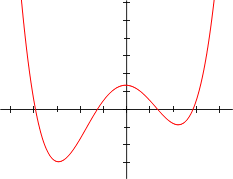
特別なケースへの対応 次の形式で表された4次方程式を考えてみましょう。1 0 x 4 + 1 1 x 3 + 1 2 x 2 + 1 3 x + 1 4 = 0 {\displaystyle a_{0}x^{4}+a_{1}x^{3}+a_{2}x^{2}+a_{3}x+a_{4}=0}
4次方程式の根を求めるための一般的な公式は存在しますが、これは主項の係数がゼロでない場合に限ります。ただし、この一般的な方法は非常に複雑で、実行時にエラーが発生しやすいため、可能であれば以下の特殊なケースのいずれかを適用するのが望ましいでしょう。
退化したケース 定数項a 4 = 0 の場合、根の 1 つはx = 0 であり、他の根はxで割って結果として得られる 三次方程式 を解くことによって見つけることができます。
1 0 x 3 + 1 1 x 2 + 1 2 x + 1 3 = 0. {\displaystyle a_{0}x^{3}+a_{1}x^{2}+a_{2}x+a_{3}=0.\,}
双二次方程式 3 と1が 0 に等しい4次方程式は次の形式をとる。
1 0 x 4 + 1 2 x 2 + 1 4 = 0 {\displaystyle a_{0}x^{4}+a_{2}x^{2}+a_{4}=0\,\!} したがって、これは双二次方程式 であり、簡単に解くことができます。z = x 2 {\displaystyle z=x^{2}}
1 0 z 2 + 1 2 z + 1 4 = 0 {\displaystyle a_{0}z^{2}+a_{2}z+a_{4}=0\,\!} これは単純な二次方程式であり、二次方程式の解の公式を使えば簡単に解を求めることができます。
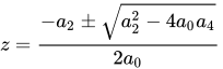
z = − 1 2 ± 1 2 2 − 4 1 0 1 4 2 1 0 {\displaystyle z={\frac {-a_{2}\pm {\sqrt {a_{2}^{2}-4a_{0}a_{4}}}}{2a_{0}}}\,\!} それを解いたとき(つまり、この2つのz 値を見つけたとき)、それらからxを抽出することができます。
x 1 = + z + {\displaystyle x_{1}=+{\sqrt {z_{+}}}\,\!} x 2 = − z + {\displaystyle x_{2}=-{\sqrt {z_{+}}}\,\!} x 3 = + z − {\displaystyle x_{3}=+{\sqrt {z_{-}}}\,\!} x 4 = − z − {\displaystyle x_{4}=-{\sqrt {z_{-}}}\,\!} z の解のいずれかが負の数または複素数である場合、x の解の一部は複素数となる。
準対称方程式 1 0 x 4 + 1 1 x 3 + 1 2 x 2 + 1 1 m x + 1 0 m 2 = 0 {\displaystyle a_{0}x^{4}+a_{1}x^{3}+a_{2}x^{2}+a_{1}mx+a_{0}m^{2}=0\,} 手順:
x 2変数変換z = x + m / x を使用します。 したがって、z 2x 2m / x ) 2m 。 これは以下のことにつながります。
1 0 ( x 2 + m 2 / x 2 ) + 1 1 ( x + m / x ) + 1 2 = 0 {\displaystyle a_{0}(x^{2}+m^{2}/x^{2})+a_{1}(x+m/x)+a_{2}=0} 1 0 ( z 2 − 2 m ) + 1 1 ( z ) + 1 2 = 0 {\displaystyle a_{0}(z^{2}-2m)+a_{1}(z)+a_{2}=0} 1 0 z 2 + 1 1 z + ( 1 2 − 2 m 1 0 ) = 0 {\displaystyle a_{0}z^{2}+a_{1}z+(a_{2}-2ma_{0})=0} ( z = x + m / x に関する二次式)
一般的なケース 単項式の場合の、4次式の係数を用いて完全に書き出した4次式の公式。その扱いにくさから、一般的には係数から最初に計算された補助変数を用いて表される。 まず、4次式をまず縮約4次式 に変換する必要があります。
四次関数への変換 させて
解こうとしている一般の4次方程式を とする。両辺をA で割る。
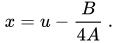
x 4 + B A x 3 + C A x 2 + D A x + E A = 0 。 {\displaystyle \ x^{4}+{B \over A}x^{3}+{C \over A}x^{2}+{D \over A}x+{E \over A}=0\ .} B がまだゼロでない場合、最初のステップはx 3 の 項を消去することです。これを行うには、変数をxから u に変更して、
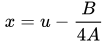
x = u − B 4 A 。 {\displaystyle \ x=u-{B \over 4A}\ .} それから
( u − B 4 A ) 4 + B A ( u − B 4 A ) 3 + C A ( u − B 4 A ) 2 + D A ( u − B 4 A ) + E A = 0 。 {\displaystyle \ \left(u-{B \over 4A}\right)^{4}+{B \over A}\left(u-{B \over 4A}\right)^{3}+{C \over A}\left(u-{B \over 4A}\right)^{2}+{D \over A}\left(u-{B \over 4A}\right)+{E \over A}=0\ .} 二項式のべき乗を展開すると
( u 4 − B A u 3 + 6 u 2 B 2 16 A 2 − 4 u B 3 64 A 3 + B 4 256 A 4 ) + B A ( u 3 − 3 u 2 B 4 A + 3 u B 2 16 A 2 − B 3 64 A 3 ) + C A ( u 2 − u B 2 A + B 2 16 A 2 ) + D A ( u − B 4 A ) + E A = 0 。 {\displaystyle \ \left(u^{4}-{B \over A}u^{3}+{6u^{2}B^{2} \over 16A^{2}}-{4uB^{3} \over 64A^{3}}+{B^{4} \over 256A^{4}}\right)+{B \over A}\left(u^{3}-{3u^{2}B \over 4A}+{3uB^{2} \over 16A^{2}}-{B^{3} \over 64A^{3}}\right)+{C \over A}\left(u^{2}-{uB \over 2A}+{B^{2} \over 16A^{2}}\right)+{D \over A}\left(u-{B \over 4A}\right)+{E \over A}=0\ .} u の同じべき乗を集めると、
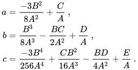
u 4 + ( − 3 B 2 8 A 2 + C A ) u 2 + ( B 3 8 A 3 − B C 2 A 2 + D A ) u + ( − 3 B 4 256 A 4 + C B 2 16 A 3 − B D 4 A 2 + E A ) = 0 。 {\displaystyle \ u^{4}+\left({-3B^{2} \over 8A^{2}}+{C \over A}\right)u^{2}+\left({B^{3} \over 8A^{3}}-{BC \over 2A^{2}}+{D \over A}\right)u+\left({-3B^{4} \over 256A^{4}}+{CB^{2} \over 16A^{3}}-{BD \over 4A^{2}}+{E \over A}\right)=0\ .} 次に、 u の係数の名前を変更します。
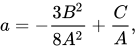
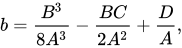
1 = − 3 B 2 8 A 2 + C A 、 b = B 3 8 A 3 − B C 2 A 2 + D A 、 c = − 3 B 4 256 A 4 + C B 2 16 A 3 − B D 4 A 2 + E A 。 {\displaystyle {\begin{aligned}a&={-3B^{2} \over 8A^{2}}+{C \over A}\ ,\\b&={B^{3} \over 8A^{3}}-{BC \over 2A^{2}}+{D \over A}\ ,\\c&={-3B^{4} \over 256A^{4}}+{CB^{2} \over 16A^{3}}-{BD \over 4A^{2}}+{E \over A}\ .\end{aligned}}} 結果として得られる方程式は
これは、縮約された4次方程式 です。
もし b = 0 {\displaystyle \ b=0\ } 次に、双二次方程式 の特殊なケースを考えますが、これは上記のように簡単に解くことができます。ただし、以下に示す一般解は、この特殊なケースには適用できないことに注意してください。 b = 0 。 {\displaystyle \ b=0\ .}
いずれの場合も、 u について縮約四次方程式を解いたら、それらの値を代入して
x = u − B 4 A {\displaystyle \ x=u-{B \over 4A}\ } 元の4次方程式を解くx の値を生成します。
b ≠ 0の場合の縮約四次方程式の解法縮退四次方程式に変換した後
u 4 + 1 u 2 + b u + c = 0 {\displaystyle u^{4}+au^{2}+bu+c=0} また、双二次方程式として解かれる特殊なケースb = 0 を除いて、ここからはb ≠ 0 であると仮定します。
左と右の用語を分けて説明します。
u 4 = − 1 u 2 − b u − c {\displaystyle u^{4}=-au^{2}-bu-c} そして両辺に、両方とも平方数 になるような項を追加します。
y を この三次方程式 の任意の解とする。
2 y 3 − 1 y 2 − 2 c y + ( 1 c − 1 4 b 2 ) = ( 2 y − 1 ) ( y 2 − c ) − 1 4 b 2 = 0 。 {\displaystyle 2y^{3}-ay^{2}-2cy+(ac-{\tfrac {1}{4}}b^{2})=(2y-a)(y^{2}-c)-{\tfrac {1}{4}}b^{2}=0\ .} すると(b ≠ 0 なので)
2 y − 1 ≠ 0 {\displaystyle 2y-a\neq 0} そこで、それで割ると、
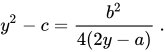
y 2 − c = b 2 4 ( 2 y − 1 ) 。 {\displaystyle y^{2}-c={\frac {b^{2}}{4(2y-a)}}\ .} それから
( u 2 + y ) 2 = u 4 + 2 y u 2 + y 2 = ( 2 y − 1 ) u 2 − b u + ( y 2 − c ) = ( 2 y − 1 ) u 2 − b u + b 2 4 ( 2 y − 1 ) = ( 2 y − 1 u − b 2 2 y − 1 ) 2 。 {\displaystyle (u^{2}+y)^{2}=u^{4}+2yu^{2}+y^{2}=(2y-a)u^{2}-bu+(y^{2}-c)=(2y-a)u^{2}-bu+{\frac {b^{2}}{\ 4(2y-a)\ }}=\left({\sqrt {2y-a\ }}\,u-{\frac {b}{2{\sqrt {2y-a\ }}}}\right)^{2}\ .} 引き算をすると、2つの平方数の差 が得られます。これは、それらの平方根の和と差の積です。
( u 2 + y ) 2 − ( 2 y − 1 u − b 2 2 y − 1 ) 2 = ( u 2 + y + 2 y − 1 u − b 2 2 y − 1 ) ( u 2 + y − 2 y − 1 u + b 2 2 y − 1 ) = 0 {\displaystyle (u^{2}+y)^{2}-\left({\sqrt {2y-a\ }}\,u-{\frac {b}{2{\sqrt {2y-a\ }}}}\right)^{2}=\left(u^{2}+y+{\sqrt {2y-a\ }}\,u-{\frac {b}{2{\sqrt {2y-a\ }}}}\right)\left(u^{2}+y-{\sqrt {2y-a\ }}\,u+{\frac {b}{2{\sqrt {2y-a\ }}}}\right)=0} これは、2つの因数それぞれに二次方程式の解の公式を適用することで解くことができます。したがって、u の取りうる値は次のとおりです。
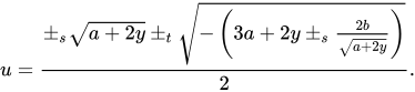
u = 1 2 ( − 2 y − 1 + − 2 y − 1 + 2 b 2 y − 1 ) 、 {\displaystyle u={\tfrac {1}{2}}\left(-{\sqrt {2y-a\ }}+{\sqrt {-2y-a+{\frac {2b}{\sqrt {2y-a\ }}}\ }}\right)\ ,} u = 1 2 ( − 2 y − 1 − − 2 y − 1 + 2 b 2 y − 1 ) 、 {\displaystyle u={\tfrac {1}{2}}\left(-{\sqrt {2y-a\ }}-{\sqrt {-2y-a+{\frac {2b}{\sqrt {2y-a\ }}}\ }}\right)\ ,} u = 1 2 ( 2 y − 1 + − 2 y − 1 − 2 b 2 y − 1 ) 、 {\displaystyle u={\tfrac {1}{2}}\left({\sqrt {2y-a\ }}+{\sqrt {-2y-a-{\frac {2b}{\sqrt {2y-a\ }}}\ }}\right)\ ,} u = 1 2 ( 2 y − 1 − − 2 y − 1 − 2 b 2 y − 1 ) 。 {\displaystyle u={\tfrac {1}{2}}\left({\sqrt {2y-a\ }}-{\sqrt {-2y-a-{\frac {2b}{\sqrt {2y-a\ }}}\ }}\right)\ .} 3次方程式の3つの根のうち別のy を用いると、同じ4つのu の値が異なる順序で現れるだけである。3次方程式の解は以下のとおりである。
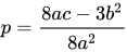
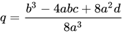
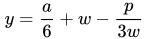
y = 1 6 + w − p 3 w {\displaystyle \ y={\frac {a}{6}}+w-{\frac {p}{3w}}\ } w = − q 2 + q 2 4 + p 3 27 3 {\displaystyle \ w={\sqrt[{3}]{-{\frac {q}{2}}+{\sqrt {{\frac {q^{2}}{4}}+{\frac {p^{3}}{27}}\ }}\ }}} 3つの可能な立方根のいずれかを使用します。賢明な戦略は、 w の絶対値が最大になるような平方根の符号を選択することです。
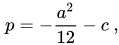
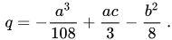
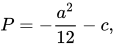
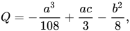
p = − 1 2 12 − c 、 {\displaystyle \ p=-{\frac {a^{2}}{12}}-c\ ,} q = − 1 3 108 + 1 c 3 − b 2 8 。 {\displaystyle \ q=-{\frac {a^{3}}{108}}+{\frac {ac}{3}}-{\frac {b^{2}}{8}}\ .}
そうでなければ、ロドヴィコ・フェラーリ が発見した方法を用いて、縮約四次方程式を解くことができる。縮約四次方程式が得られたら、次のステップは有効な恒等式を追加することである。
( u 2 + 1 ) 2 − u 4 − 2 1 u 2 = 1 2 {\displaystyle \left(u^{2}+a\right)^{2}-u^{4}-2au^{2}=a^{2}} 式(1
その結果、 u 4 の 項は( u 2 + a) 2という 完全な平方数 に折り畳まれました。2 番目の項au 2 は消えませんでしたが、符号が変わり、右辺に移動しました。
次のステップは、式( 2 y を挿入し、右辺のu2 の 係数にそれに対応する2yを挿入することです。これらの挿入を実行するために、次の有効な式が式( 2
( u 2 + 1 + y ) 2 − ( u 2 + 1 ) 2 = 2 y ( u 2 + 1 ) + y 2 = 2 y u 2 + 2 y 1 + y 2 、 {\displaystyle {\begin{aligned}(u^{2}+a+y)^{2}-(u^{2}+a)^{2}&=2y(u^{2}+a)+y^{2}\ \ \\&=2yu^{2}+2ya+y^{2},\end{aligned}}} そして
0 = ( 1 + 2 y ) u 2 − 2 y u 2 − 1 u 2 {\displaystyle 0=(a+2y)u^{2}-2yu^{2}-au^{2}\,} これら2つの式を足し合わせると、
( u 2 + 1 + y ) 2 − ( u 2 + 1 ) 2 = ( 1 + 2 y ) u 2 − 1 u 2 + 2 y 1 + y 2 ( y -挿入 ) {\displaystyle \left(u^{2}+a+y\right)^{2}-\left(u^{2}+a\right)^{2}=\left(a+2y\right)u^{2}-au^{2}+2ya+y^{2}\qquad \qquad (y{\hbox{-insertion}})\,} 式(2
( u 2 + 1 + y ) 2 + b u + c = ( 1 + 2 y ) u 2 + ( 2 y 1 + y 2 + 1 2 ) 。 {\displaystyle \left(u^{2}+a+y\right)^{2}+bu+c=\left(a+2y\right)u^{2}+\left(2ya+y^{2}+a^{2}\right).\,} これは以下と同等です
ここでの目的は、式( 3 y の値を選択することです。これは、二次関数 の判別式をゼロにすることで実現できます。これを説明するために、まず平方数を展開して二次関数に等しくしてみましょう。
( s u + t ) 2 = ( s 2 ) u 2 + ( 2 s t ) u + ( t 2 ) 。 {\displaystyle \left(su+t\right)^{2}=\left(s^{2}\right)u^{2}+\left(2st\right)u+\left(t^{2}\right).\,} 右辺の二次関数には3つの係数があります。2番目の係数を2乗し、そこから1番目と3番目の係数の積の4倍を引くとゼロになることが確認できます。
( 2 s t ) 2 − 4 ( s 2 ) ( t 2 ) = 0. {\displaystyle \left(2st\right)^{2}-4\left(s^{2}\right)\left(t^{2}\right)=0.\,} したがって、式( 3
( − b ) 2 − 4 ( 2 y + 1 ) ( y 2 + 2 y 1 + 1 2 − c ) = 0. {\displaystyle (-b)^{2}-4\left(2y+a\right)\left(y^{2}+2ya+a^{2}-c\right)=0.\,} 二項式に多項式を掛けます。
b 2 − 4 ( 2 y 3 + 5 1 y 2 + ( 4 1 2 − 2 c ) y + ( 1 3 − 1 c ) ) = 0 {\displaystyle b^{2}-4\left(2y^{3}+5ay^{2}+\left(4a^{2}-2c\right)y+\left(a^{3}-ac\right)\right)=0\,} 両辺を −4 で割り、−b 2/4 を 右に移動させます。
2 y 3 + 5 1 y 2 + ( 4 1 2 − 2 c ) y + ( 1 3 − 1 c − b 2 4 ) = 0 {\displaystyle 2y^{3}+5ay^{2}+\left(4a^{2}-2c\right)y+\left(a^{3}-ac-{\frac {b^{2}}{4}}\right)=0} 両辺を2で割る、
これはy に関する3次方程式 です。このような方程式を解くための任意の方法(例えば、簡約3次式への変換と カルダノの公式 の適用など)を用いてy を求めなさい。3つの解のうち、いずれか1つが正解となります。
4次方程式が与えられた場合
A x 4 + B x 3 + C x 2 + D x + E = 0 、 {\displaystyle Ax^{4}+Bx^{3}+Cx^{2}+Dx+E=0,\,} その解は、以下の計算によって求めることができる。
1 = − 3 B 2 8 A 2 + C A 、 {\displaystyle a=-{3B^{2} \over 8A^{2}}+{C \over A},} b = B 3 8 A 3 − B C 2 A 2 + D A 、 {\displaystyle b={B^{3} \over 8A^{3}}-{BC \over 2A^{2}}+{D \over A},} c = − 3 B 4 256 A 4 + C B 2 16 A 3 − B D 4 A 2 + E A 。 {\displaystyle c=-{3B^{4} \over 256A^{4}}+{CB^{2} \over 16A^{3}}-{BD \over 4A^{2}}+{E \over A}.} もしb = 0 、 {\displaystyle \,b=0,}
x = − B 4 A ± s − 1 ± t 1 2 − 4 c 2 (のために b = 0 のみ) 。 {\displaystyle x=-{B \over 4A}\pm _{s}{\sqrt {-a\pm _{t}{\sqrt {a^{2}-4c}} \over 2}}\qquad {\mbox{(for }}b=0{\mbox{ only)}}.} それ以外の場合は、
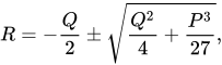
P = − 1 2 12 − c 、 {\displaystyle P=-{a^{2} \over 12}-c,} Q = − 1 3 108 + 1 c 3 − b 2 8 、 {\displaystyle Q=-{a^{3} \over 108}+{ac \over 3}-{b^{2} \over 8},} R = − Q 2 ± Q 2 4 + P 3 27 、 {\displaystyle R=-{Q \over 2}\pm {\sqrt {{Q^{2} \over 4}+{P^{3} \over 27}}},} (平方根の符号はどちらでも構いません)
U = R 3 、 {\displaystyle U={\sqrt[{3}]{R}},} (複合根は3つありますが、どれでも構いません。)
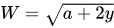
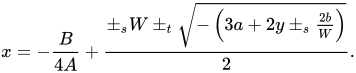
y = − 5 6 1 + { U = 0 → − Q 3 U ≠ 0 、 → U − P 3 U 、 {\displaystyle y=-{5 \over 6}a+{\begin{cases}U=0&\to -{\sqrt[{3}]{Q}}\\U\neq 0,&\to U-{P \over 3U},\end{cases}}\quad \quad \quad } W = 1 + 2 y {\displaystyle W={\sqrt {a+2y}}} x = − B 4 A + ± s W ± t − ( 3 1 + 2 y ± s 2 b W ) 2 。 {\displaystyle x=-{B \over 4A}+{\pm _{s}W\pm _{t}{\sqrt {-\left(3a+2y\pm _{s}{2b \over W}\right)}} \over 2}.} 2 つの ± s は 同じ符号でなければなりませんが、± t s t x を計算します。この式は、重複根を問題なく処理します。 フェラーリは、こうした複雑な 解法の一つを最初に発見した人物である。彼が解いた方程式は
x 4 + 6 x 2 − 60 x + 36 = 0 {\displaystyle x^{4}+6x^{2}-60x+36=0} which was already in depressed form. It has a pair of solutions which can be found with the set of formulas shown above.
If the coefficients of the quartic equation are real then the nested depressed cubic equation (5
Furthermore, the cubic function
C ( v ) = v 3 + P v + Q , {\displaystyle C(v)=v^{3}+Pv+Q,} where P and Q are given by (5
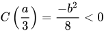
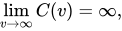
C ( a 3 ) = − b 2 8 < 0 {\displaystyle C\left({a \over 3}\right)={-b^{2} \over 8}<0} lim v → ∞ C ( v ) = ∞ , {\displaystyle \lim _{v\to \infty }C(v)=\infty ,} a {\displaystyle a} b {\displaystyle b} 1
This means that (5 a 3 {\displaystyle a \over 3} 4 − a 2 {\displaystyle -a \over 2}
Using this root the term a + 2 y {\displaystyle {\sqrt {a+2y}}} 6 6 [ 5]
Obtaining alternative solutions the hard way It could happen that one only obtained one solution through the formulae above, because not all four sign patterns are tried for four solutions, and the solution obtained is complex . It may also be the case that one is only looking for a real solution. Let x {\displaystyle x} 1 denote the complex solution. If all the original coefficients A {\displaystyle A} B {\displaystyle B} C {\displaystyle C} D {\displaystyle D} E {\displaystyle E} x {\displaystyle x} 2 which is the complex conjugate of x {\displaystyle x} 1 . If the other two roots are denoted as x {\displaystyle x} 3 and x {\displaystyle x} 4 then the quartic equation can be expressed as
( x − x 1 ) ( x − x 2 ) ( x − x 3 ) ( x − x 4 ) = 0 , {\displaystyle (x-x_{1})(x-x_{2})(x-x_{3})(x-x_{4})=0,\,} but this quartic equation is equivalent to the product of two quadratic equations:
and
Since
x 2 = x 1 ⋆ {\displaystyle x_{2}=x_{1}^{\star }} then
( x − x 1 ) ( x − x 2 ) = x 2 − ( x 1 + x 1 ⋆ ) x + x 1 x 1 ⋆ = x 2 − 2 Re ( x 1 ) x + [ Re ( x 1 ) ] 2 + [ Im ( x 1 ) ] 2 . {\displaystyle {\begin{aligned}(x-x_{1})(x-x_{2})&=x^{2}-(x_{1}+x_{1}^{\star })x+x_{1}x_{1}^{\star }\\&=x^{2}-2\operatorname {Re} (x_{1})x+[\operatorname {Re} (x_{1})]^{2}+[\operatorname {Im} (x_{1})]^{2}.\end{aligned}}} Let
a = − 2 Re ( x 1 ) , {\displaystyle a=-2\operatorname {Re} (x_{1}),} b = [ Re ( x 1 ) ] 2 + [ Im ( x 1 ) ] 2 {\displaystyle b=\left[\operatorname {Re} (x_{1})\right]^{2}+\left[\operatorname {Im} (x_{1})\right]^{2}} so that equation (9
Also let there be (unknown) variables w and v such that equation (10
Multiplying equations (11 12
Comparing equation (13
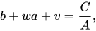
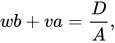
a + w = B A , {\displaystyle a+w={B \over A},} b + w a + v = C A , {\displaystyle b+wa+v={C \over A},} w b + v a = D A , {\displaystyle wb+va={D \over A},} and
v b = E A . {\displaystyle vb={E \over A}.} Therefore
w = B A − a = B A + 2 Re ( x 1 ) , {\displaystyle w={B \over A}-a={B \over A}+2\operatorname {Re} (x_{1}),} v = E A b = E A ( [ Re ( x 1 ) ] 2 + [ Im ( x 1 ) ] 2 ) . {\displaystyle v={E \over Ab}={\frac {E}{A\left(\left[\operatorname {Re} (x_{1})\right]^{2}+\left[\operatorname {Im} (x_{1})\right]^{2}\right)}}.} Equation (12 x yielding
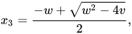
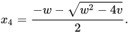
x 3 = − w + w 2 − 4 v 2 , {\displaystyle x_{3}={-w+{\sqrt {w^{2}-4v}} \over 2},} x 4 = − w − w 2 − 4 v 2 . {\displaystyle x_{4}={-w-{\sqrt {w^{2}-4v}} \over 2}.} One of these two solutions should be the desired real solution.
Alternative methods
Resolvent cubic Resolvent cubic shows how a resolvent cubic equation may be used to find the roots of a monic depressed quartic equation by finding the roots of two quadratic equations. Particularly simple is the Third Definition. Let
x 4 + c x 2 + d x + e = ( x 2 + p x + q ) ( x 2 − p x + s ) = x 4 + ( s + q − p 2 ) x 2 + p ( s − q ) x + q s ⇒ {\displaystyle {\begin{aligned}x^{4}+c\,x^{2}+d\,x+e&=(x^{2}+p\,x+q)\,(x^{2}-p\,x+s)\\&=x^{4}+(s+q-p^{2})\,x^{2}+p\,(s-q)\,x+q\,s\quad \Rightarrow \end{aligned}}}
p 2 + c = s + q d p = s − q e = q s ⇒ {\displaystyle p^{2}+c=s+q\quad \quad {\frac {d}{p}}=s-q\quad \quad e=q\,s\quad \Rightarrow }
( p 2 + c ) 2 − ( d p ) 2 = 4 e {\displaystyle (p^{2}+c)^{2}-\left({\frac {d}{p}}\right)^{2}=4\,e}
This cubic equation in p 2 {\displaystyle p^{2}} これはデカルト のレゾルベント として知られています[ 6 ] [ 7 ] ± p {\displaystyle \pm p}
適切なメビウス変換を選択すれば、4次方程式を新しい変数の2乗に関する 2次方程式 に変換できる。これは既知の方法である。[ 8 ]
このようなメビウス変換を見つけるには、三次方程式 を解く必要があり、問題が単純化されます。たとえば、先頭係数が 1 で、どちらも ない、縮小された四次方程式から始めます。1 1 {\displaystyle a_{1}} 1 0 {\displaystyle a_{0}}
x 4 + 1 2 x 2 + 1 1 x + 1 0 = 0 {\displaystyle x^{4}+a_{2}x^{2}+a_{1}x+a_{0}=0}
そしてメビウス変換を行う。
x = A + B y 1 + y {\displaystyle x={\frac {A+By}{1+y}}}
結果として得られる4次方程式の1次および3次係数をy {\displaystyle y} A + B {\displaystyle A+B}
1 1 ( A + B ) 3 + ( 4 1 0 − 2 1 1 1 2 − 1 2 2 ) ( A + B ) 2 − 2 1 1 1 2 ( A + B ) − 1 1 2 = 0 {\displaystyle a_{1}(A+B)^{3}+(4a_{0}-2a_{1}a_{2}-{a_{2}}^{2})(A+B)^{2}-2a_{1}a_{2}(A+B)-{a_{1}}^{2}=0}
そして、A + B {\displaystyle A+B} A {\displaystyle A}
2 ( A + B ) A 2 − 2 ( A + B ) 2 A − 1 2 ( A + B ) − 1 1 = 0 {\displaystyle 2(A+B)A^{2}-2(A+B)^{2}A-a_{2}(A+B)-a_{1}=0}
結果として得られる二次方程式を解くと、y 2 {\displaystyle y^{2}} y 2 {\displaystyle y^{2}} y 2 {\displaystyle y^{2}}
3次方程式A + B {\displaystyle {\textbf {A}}+{\textbf {B}}} P 2 − Q ( A + B ) 2 = 0 {\displaystyle P^{2}-Q(A+B)^{2}=0}
P ≡ b 1 − b 3 2 ( A − B ) = 2 A B ( A + B ) + 1 2 ( A + B ) + 1 1 {\displaystyle P\equiv {\frac {b_{1}-b_{3}}{2(A-B)}}=2\,A\,B\,(A+B)+a_{2}(A+B)+a_{1}}
Q ≡ B b 1 − A b 3 A − B = 4 A 2 B 2 − 1 1 ( A + B ) − 4 1 0 = 0 {\displaystyle Q\equiv {\frac {B\,b_{1}-A\,b_{3}}{A-B}}=4A^{2}B^{2}-a_{1}(A+B)-4a_{0}=0}
ここで、b i は y に関する 4 次多項式の係数です。これは、この方程式がどのように得られたかを示しています。
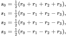
ガロア理論と因数分解 4つの要素上の対称群 S 4 は 、クライン4群を 正規部分群 として持つ。これは、根が離散フーリエ変換 または根のアダマール行列 変換として様々に記述できるレゾルベントを使用することを示唆している。iが0から3までの場合、r iが以下の根であると 仮定する 。
x 4 + b x 3 + c x 2 + d x + e = 0 ( 1 ) {\displaystyle x^{4}+bx^{3}+cx^{2}+dx+e=0\qquad (1)} ここで設定すると
s 0 = 1 2 ( r 0 + r 1 + r 2 + r 3 ) 、 s 1 = 1 2 ( r 0 − r 1 + r 2 − r 3 ) 、 s 2 = 1 2 ( r 0 + r 1 − r 2 − r 3 ) 、 s 3 = 1 2 ( r 0 − r 1 − r 2 + r 3 ) 、 {\displaystyle {\begin{aligned}s_{0}&={\tfrac {1}{2}}(r_{0}+r_{1}+r_{2}+r_{3}),\\s_{1}&={\tfrac {1}{2}}(r_{0}-r_{1}+r_{2}-r_{3}),\\s_{2}&={\tfrac {1}{2}}(r_{0}+r_{1}-r_{2}-r_{3}),\\s_{3}&={\tfrac {1}{2}}(r_{0}-r_{1}-r_{2}+r_{3}),\end{aligned}}} 変換は対合であるため、4 つの s i を用いて根を全く同じ方法で表すことができます。s 0 = − b /2 の値がわかっているので、実際には s 1 、s 2 、s 3 の値だけが必要です。これらは多項式を展開することで求めることができます。
( z 2 − s 1 2 ) ( z 2 − s 2 2 ) ( z 2 − s 3 2 ) ( 2 ) {\displaystyle \left(z^{2}-s_{1}^{2}\right)\left(z^{2}-s_{2}^{2}\right)\left(z^{2}-s_{3}^{2}\right)\qquad (2)} b = 0という単純化の仮定をすると、
z 6 + 2 c z 4 + ( c 2 − 4 e ) z 2 − d 2 ( 3 ) {\displaystyle z^{6}+2cz^{4}+\left(c^{2}-4e\right)z^{2}-d^{2}\qquad (3)} この多項式は6次ですが、z 2 に関しては3次なので、対応する方程式は解くことができます。試行錯誤によって、どの3つの根が正しいかを判断し、それによって4次方程式の解を求めることができます。
因数分解に同じレゾルベント多項式の根を使用することで、試行の要件をすべて取り除くことができます。w が (3) の任意の根である場合、そして
F 1 = x 2 + w x + 1 2 w 2 + 1 2 c − 1 2 ⋅ c 2 w d − 1 2 ⋅ w 5 d − c w 3 d + 2 e w d {\displaystyle F_{1}=x^{2}+wx+{\frac {1}{2}}w^{2}+{\frac {1}{2}}c-{\frac {1}{2}}\cdot {\frac {c^{2}w}{d}}-{\frac {1}{2}}\cdot {\frac {w^{5}}{d}}-{\frac {cw^{3}}{d}}+2{\frac {ew}{d}}} F 2 = x 2 − w x + 1 2 w 2 + 1 2 c + 1 2 ⋅ w 5 d + c w 3 d − 2 e w d + 1 2 ⋅ c 2 w d {\displaystyle F_{2}=x^{2}-wx+{\frac {1}{2}}w^{2}+{\frac {1}{2}}c+{\frac {1}{2}}\cdot {\frac {w^{5}}{d}}+{\frac {cw^{3}}{d}}-2{\frac {ew}{d}}+{\frac {1}{2}}\cdot {\frac {c^{2}w}{d}}} それから
F 1 F 2 = x 4 + c x 2 + d x + e ( 4 ) {\displaystyle F_{1}F_{2}=x^{4}+cx^{2}+dx+e\qquad \qquad (4)} したがって、w について解き、次に二次方程式の解の公式を用いて 2 つの因数の根を求めることで、4 次方程式を解くことができます。
近似法 上記の方法は、原理的には厳密な根探索法である。また、デュラン・ケルナー法 のように、根に向かって反復的に収束する逐次近似法を用いることも可能である。




































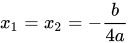

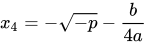
![{\displaystyle (p^{2}+12r)^{3}=[p(p^{2}-36r)+{\frac {27}{2}}q^{2}]^{2}>0\neq {q}}](https://wikimedia.org/api/rest_v1/media/math/render/svg/49aa203796648c979e086b49eaaa19579859ca83)
![{\displaystyle x={\frac {1}{2}}\left[\xi {\sqrt {s_{1}}}\pm {\sqrt {2{\biggl (}s_{2}-{\frac {\xi q}{\sqrt {s_{1}}}}{\biggr )}}}\right]-{\frac {b}{4a}}}](https://wikimedia.org/api/rest_v1/media/math/render/svg/d4975d90cce615ee12fabb813532f492ef11b82e)
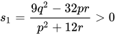
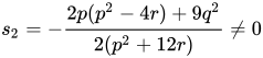

















![{\displaystyle \ w={\sqrt[{3}]{-{\frac {q}{2}}+{\sqrt {{\frac {q^{2}}{4}}+{\frac {p^{3}}{27}}\ }}\ }}}](https://wikimedia.org/api/rest_v1/media/math/render/svg/58ba0419f46e27a9676c2d9375d90bbf8808ede0)





















![{\displaystyle U={\sqrt[{3}]{R}},}](https://wikimedia.org/api/rest_v1/media/math/render/svg/20a6632a438df747a811e14058b1a34758442381)
![{\displaystyle y=-{5 \over 6}a+{\begin{cases}U=0&\to -{\sqrt[{3}]{Q}}\\U\neq 0,&\to U-{P \over 3U},\end{cases}}\quad \quad \quad }](https://wikimedia.org/api/rest_v1/media/math/render/svg/9365e6b0443948cfea7ae46544b127fe9e91a4a8)






![{\displaystyle {\begin{aligned}(x-x_{1})(x-x_{2})&=x^{2}-(x_{1}+x_{1}^{\star })x+x_{1}x_{1}^{\star }\\&=x^{2}-2\operatorname {Re} (x_{1})x+[\operatorname {Re} (x_{1})]^{2}+[\operatorname {Im} (x_{1})]^{2}.\end{aligned}}}](https://wikimedia.org/api/rest_v1/media/math/render/svg/5a5a7c94c0e25cf2ad315f1d423e9bac0251b672)

![{\displaystyle b=\left[\operatorname {Re} (x_{1})\right]^{2}+\left[\operatorname {Im} (x_{1})\right]^{2}}](https://wikimedia.org/api/rest_v1/media/math/render/svg/6f2e2d63133198833d2f455081c59991c089847d)



![{\displaystyle v={E \over Ab}={\frac {E}{A\left(\left[\operatorname {Re} (x_{1})\right]^{2}+\left[\operatorname {Im} (x_{1})\right]^{2}\right)}}.}](https://wikimedia.org/api/rest_v1/media/math/render/svg/16d32387e4d53b34398a4589257cbcf5b8a87b54)