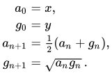
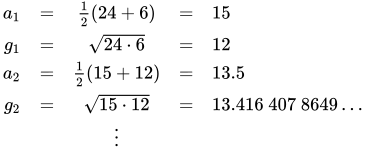
例 a 0 = 24g 0 = 61 1 = 1 2 ( 24 + 6 ) = 15 g 1 = 24 ⋅ 6 = 12 1 2 = 1 2 ( 15 + 12 ) = 13.5 g 2 = 15 ⋅ 12 = 13.416 407 8649 … ⋮ {\displaystyle {\begin{array}{rcccl}a_{1}&=&{\tfrac {1}{2}}(24+6)&=&15\\g_{1}&=&{\sqrt {24\cdot 6}}&=&12\\a_{2}&=&{\tfrac {1}{2}}(15+12)&=&13.5\\g_{2}&=&{\sqrt {15\cdot 12}}&=&13.416\ 407\ 8649\dots \\&&\vdots &&\end{array}}}
a n g n が 171 481 725 615 420 766 813 156 974 399 243 053 838 8544 [ 2 ]
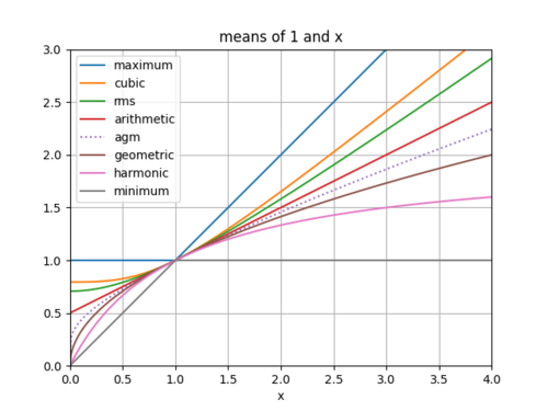
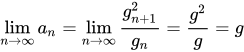
物件 2 つの正の数x とy の幾何平均と算術平均は、どちらもその 2 つの数の間にあります。( x ≠ y 厳密に その 2 つの数の間にあります。) 2 つの正の数の幾何平均は、算術平均より大きくなることはありません 。[ 3 ] g 0 ≤ g 1 ≤ g 2 ≤ ... であり、算術平均は減少数列a 0 ≥ a 1 ≥ a 2 ≥ ... であり、任意のn に対してg n ≤ M ( x , y ) ≤ a n x ≠ y
M ( x , y )はx y 、 x y
r ≥ 0 のM ( rx , ry ) = r M ( x , y )
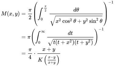
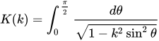
M ( x , y )[ 4 ] M ( x 、 y ) = π 2 ( ∫ 0 π 2 d θ x 2 コス 2 θ + y 2 罪 2 θ ) − 1 = π ( ∫ 0 ∞ d t t ( t + x 2 ) ( t + y 2 ) ) − 1 = π 4 ⋅ x + y K ( x − y x + y ) {\displaystyle {\begin{aligned}M(x,y)&={\frac {\pi }{2}}\left(\int _{0}^{\frac {\pi }{2}}{\frac {d\theta }{\sqrt {x^{2}\cos ^{2}\theta +y^{2}\sin ^{2}\theta }}}\right)^{-1}\\&=\pi \left(\int _{0}^{\infty }{\frac {dt}{\sqrt {t(t+x^{2})(t+y^{2})}}}\right)^{-1}\\&={\frac {\pi }{4}}\cdot {\frac {x+y}{K\left({\frac {xy}{x+y}}\right)}}\end{aligned}}} K ( k )は第一種完全楕円積分 である。K ( k ) = ∫ 0 π 2 d θ 1 − k 2 罪 2 θ {\displaystyle K(k)=\int _{0}^{\frac {\pi }{2}}{\frac {d\theta }{\sqrt {1-k^{2}\sin ^{2}\theta }}}} 楕円フィルタ 設計で使用される楕円積分を計算する効率的な方法を提供する。[ 5 ]
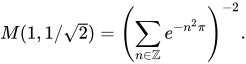
算術平均と幾何平均はヤコビのシータ関数と関連している。 θ 3 \displaystyle \theta _{3}} 6 ] M ( 1 、 x ) = θ 3 − 2 ( exp ( − π M ( 1 、 x ) M ( 1 、 1 − x 2 ) ) ) = ( ∑ n ∈ Z exp ( − n 2 π M ( 1 、 x ) M ( 1 、 1 − x 2 ) ) ) − 2 、 {\displaystyle M(1,x)=\theta _{3}^{-2}\left(\exp \left(-\pi {\frac {M(1,x)}{M\left(1,{\sqrt {1-x^{2}}}\right)}}\right)\right)=\left(\sum _{n\in \mathbb {Z} }\exp \left(-n^{2}\pi {\frac {M(1,x)}{M\left(1,{\sqrt {1-x^{2}}}\right)}}\right)\right)^{-2},} x = 1 / 2 {\displaystyle x=1/{\sqrt {2}}} M ( 1 、 1 / 2 ) = ( ∑ n ∈ Z e − n 2 π ) − 2 。 {\displaystyle M(1,1/{\sqrt {2}})=\left(\sum _{n\in \mathbb {Z} }e^{-n^{2}\pi }\right)^{-2}.}
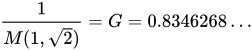
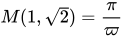
1と2の平方根 の算術平均と幾何平均の逆数はガウス定数 である。1 M ( 1 、 2 ) = G = 0.8346268 … \displaystyle {\frac {1}{M(1,{\sqrt {2}})}}=G=0.8346268\dots } [ 注1 ] M ( 1 、 2 ) = π ϖ {\displaystyle M(1,{\sqrt {2}})={\frac {\pi }{\varpi }}} ϖ {\displaystyle \varpi } はレムニスケート定数 です。
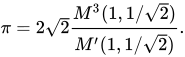
1941年、M ( 1 、 2 ) {\displaystyle M(1,{\sqrt {2}})} G {\displaystyle G} テオドール・シュナイダー によって超越的であること が証明された。[ 注2 ] [ 7 ] [ 8 ] { π 、 M ( 1 、 1 / 2 ) } {\displaystyle \{\pi ,M(1,1/{\sqrt {2}})\}} 代数的 に独立しているQ {\displaystyle \mathbb {Q} } 9 ] [ 10 ] は { π 、 M ( 1 、 1 / 2 ) 、 M ′ ( 1 、 1 / 2 ) } {\displaystyle \{\pi ,M(1,1/{\sqrt {2}}),M'(1,1/{\sqrt {2}})\}} 導関数を表す)は代数的に独立ではない Q {\displaystyle \mathbb {Q} } [ 11 ] π = 2 2 M 3 ( 1 、 1 / 2 ) M ′ ( 1 、 1 / 2 ) 。 {\displaystyle \pi =2{\sqrt {2}}{\frac {M^{3}(1,1/{\sqrt {2}})}{M'(1,1/{\sqrt {2}})}}.} 平均と調和平均GH は、幾何平均と 調和 平均の類似した数列を使用して計算でき、実際にはGH( x , y ) = 1/ M (1/ x , 1/ y ) = xy / M ( x , y ) となります。[ 12 ] は幾何平均と同等です 。
算術平均と幾何平均は、とりわけ対数 、 第一種および第二種の完全および不完全楕円積分 [ 13 ] ヤコビ楕円関数 [ 14 ]
この証明はガウスによって与えられた 。[ 1 ]
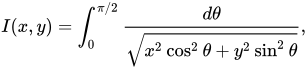
私 ( x 、 y ) = ∫ 0 π / 2 d θ x 2 コス 2 θ + y 2 罪 2 θ 、 {\displaystyle I(x,y)=\int _{0}^{\pi /2}{\frac {d\theta }{\sqrt {x^{2}\cos ^{2}\theta +y^{2}\sin ^{2}\theta }}},}
積分変数を変更するθ ′ {\displaystyle \theta '}
罪 θ = 2 x 罪 θ ′ ( x + y ) + ( x − y ) 罪 2 θ ′ ⇒ d ( 罪 θ ) = d ( 2 x 罪 θ ′ ( x + y ) + ( x − y ) 罪 2 θ ′ ) ⇒ コス θ d θ = 2 x ( x + y ) − ( x − y ) 罪 2 θ ′ ( ( x + y ) + ( x − y ) 罪 2 θ ′ ) 2 コス θ ′ d θ ′ {\displaystyle {\begin{aligned}\sin \theta &={\frac {2x\sin \theta '}{(x+y)+(xy)\sin ^{2}\theta '}}\\\Rightarrow d(\sin \theta )&=d\left({\frac {2x\sin \theta '}{(x+y)+(xy)\sin ^{2}\theta '}}\right)\\\Rightarrow \cos \theta \ d\theta &=2x{\frac {(x+y)-(xy)\sin ^{2}\theta '}{((x+y)+(xy)\sin ^{2}\theta ')^{2}}}\ \cos \theta 'd\theta '\end{aligned}}}
コス θ = ( x + y ) 2 − 2 ( x 2 + y 2 ) 罪 2 θ ′ + ( x − y ) 2 罪 4 θ ′ ( x + y ) + ( x − y ) 罪 2 θ ′ = コス θ ′ ( x − y ) 2 コス 2 θ ′ + 4 x y ( x + y ) + ( x − y ) 罪 2 θ ′ = コス θ ′ ( x + y ) 2 コス 2 θ ′ + 4 x y 罪 2 θ ′ ( x + y ) + ( x − y ) 罪 2 θ ′ 、 {\displaystyle {\begin{aligned}\cos \theta &={\frac {\sqrt {(x+y)^{2}-2(x^{2}+y^{2})\sin ^{2}\theta '+(x-y)^{2}\sin ^{4}\theta '}}{(x+y)+(x-y)\sin ^{2}\theta '}}\\&={\frac {\cos \theta '{\sqrt {(x-y)^{2}\cos ^{2}\theta '+4xy}}}{(x+y)+(x-y)\sin ^{2}\theta '}}\\&={\frac {\cos \theta '{\sqrt {(x+y)^{2}\cos ^{2}\theta '+4xy\sin ^{2}\theta '}}}{(x+y)+(x-y)\sin ^{2}\theta '}},\end{aligned}}}
⇒ コス θ d θ = コス θ ′ ( x + y ) 2 コス 2 θ ′ + 4 x y 罪 2 θ ′ ( x + y ) + ( x − y ) 罪 2 θ ′ d θ = 2 x ( x + y ) − ( x − y ) 罪 2 θ ′ ( ( x + y ) + ( x − y ) 罪 2 θ ′ ) 2 コス θ ′ d θ ′ 、 {\displaystyle \Rightarrow \cos \theta \ d\theta ={\frac {\cos \theta '{\sqrt {(x+y)^{2}\cos ^{2}\theta '+4xy\sin ^{2}\theta '}}}{(x+y)+(x-y)\sin ^{2}\theta '}}\ d\theta =2x{\frac {(x+y)-(x-y)\sin ^{2}\theta '}{((x+y)+(x-y)\sin ^{2}\theta ')^{2}}}\ \cos \theta 'd\theta ',}
⇒ d θ = x ( ( x + y ) − ( x − y ) 罪 2 θ ′ ) ( ( x + y ) + ( x − y ) 罪 2 θ ′ ) 2 d θ ′ ( x + y ) 2 コス 2 θ ′ + 4 x y 罪 2 θ ′ 、 {\displaystyle \Rightarrow d\theta ={\frac {x((x+y)-(x-y)\sin ^{2}\theta ')}{((x+y)+(x-y)\sin ^{2}\theta ')}}{\frac {2d\theta '}{\sqrt {(x+y)^{2}\cos ^{2}\theta '+4xy\sin ^{2}\theta '}}}\ ,}
x 2 コス 2 θ + y 2 罪 2 θ = x 2 ( ( x + y ) 2 − 2 ( x 2 + y 2 ) 罪 2 θ ′ + ( x − y ) 2 罪 4 θ ′ ) + 4 x 2 y 2 罪 2 θ ′ ( ( x + y ) + ( x − y ) 罪 2 θ ′ ) = x ( ( x + y ) − ( x − y ) 罪 2 θ ′ ) ( ( x + y ) + ( x − y ) 罪 2 θ ′ ) {\displaystyle {\begin{aligned}{\sqrt {x^{2}\cos ^{2}\theta +y^{2}\sin ^{2}\theta }}&={\frac {\sqrt {x^{2}((x+y)^{2}-2(x^{2}+y^{2})\sin ^{2}\theta '+(x-y)^{2}\sin ^{4}\theta ')+4x^{2}y^{2}\sin ^{2}\theta '}}{((x+y)+(x-y)\sin ^{2}\theta ')}}\\&={\frac {x((x+y)-(x-y)\sin ^{2}\theta ')}{((x+y)+(x-y)\sin ^{2}\theta ')}}\end{aligned}}}
これにより、 d θ x 2 コス 2 θ + y 2 罪 2 θ = 2 d θ ′ ( x + y ) 2 コス 2 θ ′ + 4 x y 罪 2 θ ′ = d θ ′ ( ( x + y 2 ) 2 コス 2 θ ′ + ( x y ) 2 罪 2 θ ′ 、 {\displaystyle {\frac {d\theta }{\sqrt {x^{2}\cos ^{2}\theta +y^{2}\sin ^{2}\theta }}}={\frac {2d\theta '}{\sqrt {(x+y)^{2}\cos ^{2}\theta '+4xy\sin ^{2}\theta '}}}={\frac {d\theta '}{\sqrt {(({\frac {x+y}{2}})^{2}\cos ^{2}\theta '+({\sqrt {xy}})^{2}\sin ^{2}\theta '}}},}
与える
私 ( x 、 y ) = ∫ 0 π / 2 d θ ′ ( ( x + y 2 ) 2 コス 2 θ ′ + ( x y ) 2 罪 2 θ ′ = 私 ( x + y 2 、 x y ) 。 {\displaystyle {\begin{aligned}I(x,y)&=\int _{0}^{\pi /2}{\frac {d\theta '}{\sqrt {(({\frac {x+y}{2}})^{2}\cos ^{2}\theta '+({\sqrt {xy}})^{2}\sin ^{2}\theta '}}}\\&=I{\bigl (}{\tfrac {x+y}{2}},{\sqrt {xy}}{\bigr )}.\end{aligned}}}
したがって、
私 ( x 、 y ) = 私 ( 1 1 、 g 1 ) = 私 ( 1 2 、 g 2 ) = ⋯ = 私 ( M ( x 、 y ) 、 M ( x 、 y ) ) = π / ( 2 M ( x 、 y ) ) 。 {\displaystyle {\begin{aligned}I(x,y)&=I(a_{1},g_{1})=I(a_{2},g_{2})=\cdots \\&=I{\bigl (}M(x,y),M(x,y){\bigr )}=\pi /{\bigr (}2M(x,y){\bigl )}.\end{aligned}}} 私 ( z 、 z ) = π / ( 2 z ) {\displaystyle I(z,z)=\pi /(2z)}
最終的に、望ましい結果が得られる。
M ( x 、 y ) = π / ( 2 私 ( x 、 y ) ) 。 {\displaystyle M(x,y)=\pi /{\bigl (}2I(x,y){\bigr )}.}
アプリケーション
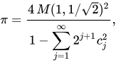
π ガウス・ルジャンドルアルゴリズム によれば、[ 15 ]
π = 4 M ( 1 、 1 / 2 ) 2 1 − ∑ j = 1 ∞ 2 j + 1 c j 2 、 {\displaystyle \pi ={\frac {4\,M(1,1/{\sqrt {2}})^{2}}{1-\displaystyle \sum _{j=1}^{\infty }2^{j+1}c_{j}^{2}}},}
どこ
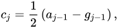
c j = 1 2 ( 1 j − 1 − g j − 1 ) 、 {\displaystyle c_{j}={\frac {1}{2}}\left(a_{j-1}-g_{j-1}\right),}
と1 0 = 1 {\displaystyle a_{0}=1} g 0 = 1 / 2 {\displaystyle g_{0}=1/{\sqrt {2}}}
c j = c j − 1 2 4 1 j 。 {\displaystyle c_{j}={\frac {c_{j-1}^{2}}{4a_{j}}}.}
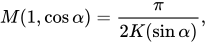
K (sin α )取1 0 = 1 {\displaystyle a_{0}=1} g 0 = コス α {\displaystyle g_{0}=\cos \alpha }
M ( 1 、 コス α ) = π 2 K ( 罪 α ) 、 {\displaystyle M(1,\cos \alpha )={\frac {\pi }{2K(\sin \alpha )}},}
ここで、K ( k )は第一種 完全楕円積分である。
K ( k ) = ∫ 0 π / 2 ( 1 − k 2 罪 2 θ ) − 1 / 2 d θ 。 {\displaystyle K(k)=\int _{0}^{\pi /2}(1-k^{2}\sin ^{2}\theta )^{-1/2}\,d\theta .}
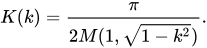
つまり、この四半期期間は AGMを通じて効率的に計算できるということです。 K ( k ) = π 2 M ( 1 、 1 − k 2 ) 。 {\displaystyle K(k)={\frac {\pi }{2M(1,{\sqrt {1-k^{2}}})}}.}
参考文献
引用文献 1 2 3 4 デビッド・コックス(1984 年 1 月)。「ガウスの算術幾何平均」。L'Enseignement Mathématique 。30 (2): 275 – 330. ↑ agm(24, 6) at Wolfram Alpha ↑ Bullen, PS (2003). "算術平均、幾何平均、調和平均". 平均とその不等式ハンドブック . ドルドレヒト: Springer Netherlands. pp. 60–174 . doi : 10.1007/978-94-017-0399-4_2 . ISBN 978-90-481-6383-0 2023年12月11日 に取得 。↑ Carson, BC (2010). "楕円積分" . Olver, Frank WJ ; Lozier, Daniel M.; Boisvert, Ronald F.; Clark, Charles W. (編). NIST 数学関数ハンドブック . Cambridge University Press. ISBN 978-0-521-19225-5 . MR 2723248 . 。 ↑ ディモポウロス、ヘラクレス G. (2011). アナログ電子フィルタ:理論、設計、合成 . Springer. pp. 147–155 . ISBN 978-94-007-2189-0 。↑ ボルウェイン、ジョナサン M.、ボルウェイン、ピーター B. (1987). 円周率と AGM: 解析的数論と計算複雑性に関する研究 (初版 ). Wiley-Interscience. ISBN 0-471-83138-7 。↑ テオドール・シュナイダー(1941年)。 「Zur Theorie der Abelschen Funktionen und Integrale」 。 数学に関するジャーナル 。 183 (19): 110–128 . 土井 : 10.1515/crll.1941.183.110 。 S2CID 118624331 。 ↑ Todd, John (1975). "The Lemniscate Constants" . Communications of the ACM . 18 (1): 14– 19. doi : 10.1145/360569.360580 . S2CID 85873 . ↑ GV Choodnovsky:解析関数に関連する定数の代数的独立性 、AMS通知22、1975年、p. A-486 ↑ GV チュドノフスキー:『超越数の理論への貢献』 、アメリカ数学会、1984年、6ページ ↑ ボルウェイン、ジョナサン M.、ボルウェイン、ピーター B. (1987). 円周率と AGM: 解析的数論と計算複雑性に関する研究 (初版 ). Wiley-Interscience. ISBN 0-471-83138-7 。↑ Newman, DJ (1985). "BrentとSalaminの高速アルゴリズムの簡略版". Mathematics of Computation . 44 (169): 207–210 . doi : 10.2307/2007804 . JSTOR 2007804 . ↑ アブラモウィッツ、ミルトン ; ステガン、アイリーン ・アン編(1983年)[1964年6月]。 「第17章」 。 『数式、グラフ、数表付き数学関数ハンドブック』 。応用数学シリーズ。第 55巻(第10版(1972年12月)の修正を加えた第9版再版;初版 )。ワシントンDC;ニューヨーク:米国商務省国立標準局;ドーバー出版。598 ~ 599ページ 。ISBN 978-0-486-61272-0 . LCCN 64-60036 . MR 0167642 . LCCN 65-12253 . ↑ キング、ルイス V. (1924). 楕円関数と楕円積分の直接数値計算について . ケンブリッジ大学出版局. ↑ Salamin, Eugene (1976). "算術平均と幾何平均 を 用いたπの計算" . Mathematics of Computation . 30 (135): 565–570 . doi : 10.2307/2005327 . JSTOR 2005327. MR 0404124 . ↑ ランデン、ジョン (1775)。「2 つの楕円弧を用いて任意の円錐双曲線の任意の弧の長さを求める一般定理の調査、およびそこから導かれるいくつかの新しい有用な定理」。 王立 協会の哲学的トランザクション 。65 : 283– 289。doi : 10.1098 / rstl.1775.0028 。S2CID 186208828 。 ↑ Brent , Richard P. (1976). "Fast Multiple-Precision Evaluation of Elementary Functions" . Journal of the ACM . 23 (2): 242–251 . CiteSeerX 10.1.1.98.4721 . doi : 10.1145/321941.321944 . MR 0395314. S2CID 6761843 . ↑ ボーウェイン、ジョナサン M. ; ボーウェイン、ピーター B. (1987). 円周率と AGM . ニューヨーク: ワイリー. ISBN 0-471-83138-7 MR 0877728 .