米田補題

数学において、米田の補題は圏論における基本的な結果である。^{[1]これは、}固定されたオブジェクトへの型射の関数に関する抽象的な結果である。これは、群論（群をただ1つのオブジェクトと同型のみを持つミニチュア圏とみなす）からのケイリーの定理の広範な一般化である。これは、任意の局所的に小さな圏を、その圏で定義された関数（反変集合値関数）の圏に埋め込むことを可能にする。これはまた、表現可能な関数とその自然変換の埋め込まれた圏が、より大きな関数圏の他のオブジェクトとどのように関係するかを明らかにする。これは、代数幾何学と表現論におけるいくつかの現代的な発展の基礎となる重要なツールである。これは米田信夫にちなんで名付けられている。

米田の補題は、局所的に小さいカテゴリ を研究する代わりに、へのすべての関数のカテゴリ(関数を射とする集合のカテゴリ) を研究すべきであることを示唆しています。は私たちがよく理解していると思われるカテゴリであり、への関数は、既知の構造による の「表現」と見なすことができます。 元のカテゴリはこの関数カテゴリに含まれていますが、 には存在せず「隠されていた」新しいオブジェクトが関数カテゴリに現れます。 これらの新しいオブジェクトを古いオブジェクトと同じように扱うと、理論が統一され、単純化されることがよくあります。 ${\displaystyle {\mathcal {C}}}$${\displaystyle {\mathcal {C}}}$${\displaystyle \mathbf {集合} }$${\displaystyle \mathbf {集合} }$${\displaystyle {\mathcal {C}}}$${\displaystyle \mathbf {集合} }$${\displaystyle {\mathcal {C}}}$${\displaystyle {\mathcal {C}}}$${\displaystyle {\mathcal {C}}}$

このアプローチは、環上の加群を調べることによって環を研究する一般的な方法に似ています (実際、これを一般化しています) 。環はカテゴリ の代わりになり、環上の加群のカテゴリは 上で定義される関数のカテゴリです。 ${\displaystyle {\mathcal {C}}}$${\displaystyle {\mathcal {C}}}$

米田の補題は、固定されたカテゴリから集合のカテゴリへの関数に関するものです。が局所的に小さなカテゴリである場合（つまり、hom-集合が実際の集合であり、適切なクラスではない場合）、 の各オブジェクトは、hom-関数と呼ばれる自然な関数を に生じます。 この関数は次のように表されます。 ${\displaystyle {\mathcal {C}}}$${\displaystyle \mathbf {集合} }$${\displaystyle {\mathcal {C}}}$${\displaystyle A}$${\displaystyle {\mathcal {C}}}$${\displaystyle \mathbf {集合} }$

${\displaystyle h_{A}=\mathrm {Hom} (A,-)}$。

(共変)ホム関手は射の集合に射(ただし)を送り、 の射 (左側にとの合成)に射 (ただし ) を送り、その射はの射に の射を送ります。つまり、 ${\displaystyle h_{A}}$${\displaystyle X\in {\mathcal {C}}}$ ${\displaystyle \mathrm {ホム} (A,X)}$${\displaystyle f\colon X\to Y}$${\displaystyle Y\in {\mathcal {C}}}$${\displaystyle f\circ -}$${\displaystyle f}$${\displaystyle g}$${\displaystyle \mathrm {ホム} (A,X)}$${\displaystyle f\circ g}$${\displaystyle \mathrm {ホム} (A,Y)}$

${\displaystyle h_{A}(f)=\mathrm {Hom} (A,f),{\text{ または}}}$

${\displaystyle h_{A}(f)(g)=f\circ g}$

米田の補題はこう述べています:

ここで、表記はから までの関数のカテゴリを表します。 ${\displaystyle \mathbf {集合} ^{\mathcal {C}}}$${\displaystyle {\mathcal {C}}}$${\displaystyle \mathbf {集合} }$

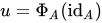
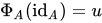
からへの自然変換が与えられた場合、 の対応する要素は です。^[a]の要素が与えられた場合、 に対応する自然変換は によって与えられ、これはの値を射に割り当てます。 ${\displaystyle \Phi}$${\displaystyle h_{A}}$${\displaystyle F}$${\displaystyle F(A)}$${\displaystyle u=\ファイ _{A}(\mathrm {id} _{A})}$${\displaystyle u}$${\displaystyle F(A)}$${\displaystyle \Phi _{X}(f)=F(f)(u)}$${\displaystyle f\colon A\to X}$${\displaystyle F(X)}$

^{米田の補題[2]}には反変版があり、これはから への反変関手に関するものである。この版では反変ホム関手 ${\displaystyle {\mathcal {C}}}$${\displaystyle \mathbf {集合} }$

${\displaystyle h^{A}=\mathrm {Hom} (-,A),}$

これはホム集合 に送られる。からへの任意の反変関手が与えられたとき、米田の補題は次のように主張する。 ${\displaystyle X}$${\displaystyle \mathrm {Hom} (X,A)}$${\displaystyle G}$${\displaystyle {\mathcal {C}}}$${\displaystyle \mathbf {集合} }$

${\displaystyle \mathrm {Nat} (h^{A},G)\cong G(A).}$

（共変）米田補題（各およびに対して）で与えられる全単射は、からまでの２つの特定の関手間の自然な同型性の成分である。^{[3] ： 61}２つの関手のうちの１つは評価関手である。 ${\displaystyle A}$${\displaystyle F}$${\displaystyle {\mathcal {C}}\times \mathbf {Set} ^{\mathcal {C}}}$${\displaystyle \mathbf {集合} }$

${\displaystyle -(-)\colon {\mathcal {C}}\times \mathbf {Set} ^{\mathcal {C}}\to \mathbf {Set} }$

${\displaystyle -(-)\colon (A,F)\mapsto F(A)}$

写像のペアと写像への 自然変換を送る${\displaystyle (f,\Phi )}$${\displaystyle f\colon A\to B}$${\displaystyle {\mathcal {C}}}$ ${\displaystyle \Phi \colon F\to G}$

${\displaystyle \Phi _{B}\circ F(f)=G(f)\circ \Phi _{A}\colon F(A)\to G(B).}$

これは、自然な同型性がわかっているので、もう一方の関手を決定するのに十分である。2番目の関手の下では

${\displaystyle \operatorname {Nat} (\hom(-,-),-)\colon {\mathcal {C}}\times \operatorname {Set} ^{\mathcal {C}}\to \operatorname {Set} ,}$

${\displaystyle \operatorname {Nat} (\hom(-,-),-)\colon (A,F)\mapsto \operatorname {Nat} (\hom(A,-),F),}$

ペアのイメージは地図です ${\displaystyle (f,\Phi )}$

${\displaystyle \operatorname {Nat} (\hom(f,-),\Phi )=\operatorname {Nat} (\hom(B,-),\Phi )\circ \operatorname {Nat} (\hom(f) ,-),F)=\オペレーター名 {Nat} (\hom(f,-),G)\circ \オペレーター名 {Nat} (\hom(A,-),\ファイ )}$

これは、自然変換を自然変換に送信し、そのコンポーネントは ${\displaystyle \Psi \colon \hom(A,-)\to F}$${\displaystyle \Phi \circ \Psi \circ \hom(f,-)\colon \hom(B,-)\to G}$

${\displaystyle (\Phi \circ \Psi \circ \hom(f,-))_{C}(g)=(\Phi \circ \Psi )_{C}(g\circ f)\qquad (g\colon B\to C).}$

共変ホム関手に対する の使用と反変ホム関手に対する の使用は完全に標準的ではありません。多くのテキストや記事では、これら 2 つの関手に対して反対の慣例を使用するか、まったく無関係な記号を使用しています。ただし、アレクサンダー・グロタンディークの基礎 EGA に始まるほとんどの現代代数幾何学のテキストでは、この記事の慣例を使用しています。^[b]${\displaystyle h_{A}}$${\displaystyle h^{A}}$

「何かに落ちる」という記憶法は、 が共変ホム関数であることを覚えておくのに役立ちます。文字が下降している場合(つまり、下付き文字の場合)、はからへの射をオブジェクトに割り当てます。 ${\displaystyle h_{A}}$${\displaystyle A}$${\displaystyle h_{A}}$${\displaystyle X}$${\displaystyle A}$ ${\displaystyle X}$

は自然変換なので、次の可換図が成り立ちます。 ${\displaystyle \Phi}$

この図は、自然変換がによって完全に決定されることを示している。なぜなら、各射に対して、 ${\displaystyle \Phi}$${\displaystyle \Phi _{A}(\mathrm {id} _{A})=u}$${\displaystyle f\colon A\to X}$

${\displaystyle \Phi _{X}(f)=(Ff)u.}$

さらに、任意の要素はこのようにして自然変換を定義します。反変の場合の証明も完全に類似しています。^[1]${\displaystyle u\in F(A)}$

米田の補題の重要な特殊ケースは、から への関数が別のホム関数である場合である。この場合、米田の補題の共変バージョンは次のように述べる。 ${\displaystyle F}$${\displaystyle {\mathcal {C}}}$${\displaystyle \mathbf {集合} }$${\displaystyle h_{B}}$

${\displaystyle \mathrm {Nat} (h_{A},h_{B})\cong \mathrm {Hom} (B,A).}$

つまり、hom 関数間の自然変換は、関連付けられたオブジェクト間の射（逆方向）と 1 対 1 に対応します。射が与えられた場合、関連付けられた自然変換は と表されます。 ${\displaystyle f\colon B\to A}$${\displaystyle \mathrm {ホム} (f,-)}$

の各オブジェクトをそれに関連付けられた hom 関手にマッピングし、各射を対応する自然変換にマッピングすると、から への反変関手、つまりから のすべての (共変) 関手の関手カテゴリが決定されます。 は共変関手として解釈できます。 ${\displaystyle A}$${\displaystyle {\mathcal {C}}}$${\displaystyle h_{A}=\mathrm {Hom} (A,-)}$${\displaystyle f\colon B\to A}$${\displaystyle \mathrm {ホム} (f,-)}$${\displaystyle h_{\bullet}}$${\displaystyle {\mathcal {C}}}$${\displaystyle \mathbf {集合} ^{\mathcal {C}}}$${\displaystyle {\mathcal {C}}}$${\displaystyle \mathbf {集合} }$${\displaystyle h_{\bullet}}$

${\displaystyle h_{\bullet }\colon {\mathcal {C}}^{\text{op}}\to \mathbf {Set} ^{\mathcal {C}}.}$

この設定における米田の補題の意味は、関数 は完全に忠実であり、したがって関数 のカテゴリにの埋め込みを に与えるということです。すべての関数 のコレクションはのサブカテゴリです。したがって、米田の埋め込みは、カテゴリ がカテゴリ に同型であることを意味します。 ${\displaystyle h_{\bullet}}$${\displaystyle {\mathcal {C}}^{\mathrm {op} }}$${\displaystyle \mathbf {集合} }$${\displaystyle \{h_{A}|A\in C\}}$${\displaystyle \mathbf {集合} ^{\mathcal {C}}}$${\displaystyle {\mathcal {C}}^{\mathrm {op} }}$${\displaystyle \{h_{A}|A\in C\}}$

米田の補題の反変版は、

${\displaystyle \mathrm {Nat} (h^{A},h^{B})\cong \mathrm {Hom} (A,B)。}$

したがって、から への共変関手が反変関手のカテゴリに生じます。 ${\displaystyle h^{\bullet}}$${\displaystyle {\mathcal {C}}}$${\displaystyle \mathbf {集合} }$

${\displaystyle h^{\bullet }\colon {\mathcal {C}}\to \mathbf {Set} ^{{\mathcal {C}}^{\mathrm {op} }}.}$

米田の補題によれば、任意の局所的に小さなカテゴリは、を介して から への反変関数のカテゴリに埋め込むことができます。これは、米田埋め込みと呼ばれます。 ${\displaystyle {\mathcal {C}}}$${\displaystyle {\mathcal {C}}}$${\displaystyle \mathbf {Set} }$${\displaystyle h^{\bullet }}$

米田埋め込みは「よ」（ひらがな ）と表記されることもある。^[4]

米田埋め込みは、本質的には、あらゆる（局所的に小さい）カテゴリに対して、そのカテゴリ内のオブジェクトは、完全かつ忠実な方法で前層によって表現できることを示しています。つまり、

${\displaystyle \mathrm {Nat} (h^{A},P)\cong P(A)}$

プレシェーフPに対して、多くの一般的なカテゴリは実際にはプレシェーフのカテゴリであり、より詳しく調べると、層のカテゴリであることがわかります。このような例は一般的に位相的な性質を持っているため、一般にトポイであると見ることができます。米田の補題は、カテゴリの位相構造を研究して理解するためのてこ点を提供します。

2つのカテゴリと2つの関数が与えられた場合、それらの間の自然な変換は次のように記述できます。^[5]${\displaystyle \mathbf {C} }$${\displaystyle \mathbf {D} }$${\displaystyle F,G:\mathbf {C} \to \mathbf {D} }$

${\displaystyle \mathrm {Nat} (F,G)=\int _{c\in \mathbf {C} }\mathrm {Hom} _{\mathbf {D} }(Fc,Gc)}$

任意の関数に対して、以下の式はすべて米田の補題の定式化である。^[6]${\displaystyle K\colon \mathbf {C} ^{op}\to \mathbf {Sets} }$${\displaystyle H\colon \mathbf {C} \to \mathbf {Sets} }$

${\displaystyle K\cong \int ^{c\in \mathbf {C} }Kc\times \mathrm {Hom} _{\mathbf {C} }(-,c),\qquad K\cong \int _{c\in \mathbf {C} }(Kc)^{\mathrm {Hom} _{\mathbf {C} }(c,-)},}$

${\displaystyle H\cong \int ^{c\in \mathbf {C} }Hc\times \mathrm {Hom} _{\mathbf {C} }(c,-),\qquad H\cong \int _{c\in \mathbf {C} }(Hc)^{\mathrm {Hom} _{\mathbf {C} }(-,c)}.}$

前加法カテゴリは、射集合がアーベル群を形成し、射の合成が双線型であるカテゴリです。例としては、アーベル群またはモジュールのカテゴリがあります。前加法カテゴリでは、射の「乗算」と「加算」の両方が存在するため、前加法カテゴリは環の一般化と見なされます。環は、1 つのオブジェクトを持つ前加法カテゴリです。

米田の補題は、元のカテゴリからアーベル群のカテゴリへの加法反変関手のカテゴリを拡張として選択すると、前加法カテゴリに対しても成り立ちます。これらは、射の加算と互換性のある関手であり、元のカテゴリ上の加法カテゴリを形成するものと考えるべきものです。米田の補題は、前加法カテゴリを拡大して、拡大バージョンが前加法のままになるようにする自然な手順をもたらします。実際、拡大バージョンはアーベルカテゴリであり、これははるかに強力な条件です。環 の場合、拡張されたカテゴリは上のすべての右加法のカテゴリであり、米田の補題のステートメントは、よく知られている同型 ${\displaystyle R}$${\displaystyle R}$

${\displaystyle M\cong \mathrm {Hom} _{R}(R,M)}$以上の   すべての適切なモジュールについて。${\displaystyle M}$${\displaystyle R}$

上で述べたように、米田の補題は群論からのケイリーの定理の広範な一般化と見なすことができます。これを理解するために、を単一のオブジェクトを持つカテゴリとし、すべての射が同型（つまり、 1つのオブジェクトを持つ群）であるとします。すると、合成の操作によってグループが形成され、任意のグループはこのようにカテゴリとして実現できます。 ${\displaystyle {\mathcal {C}}}$${\displaystyle *}$${\displaystyle G=\mathrm {Hom} _{\mathcal {C}}(*,*)}$

この文脈では、共変関数は集合と群準同型で構成されます。ここではの順列の群です。言い換えると、はG 集合です。このような関数間の自然変換は、 -集合間の同変写像と同じものです。つまり、およびのすべての に対して となる特性を持つ集合関数です。(この式の左側では、 はへのの作用を表し、右側では への の作用を表します。) ${\displaystyle {\mathcal {C}}\to \mathbf {Set} }$${\displaystyle X}$ ${\displaystyle G\to \mathrm {Perm} (X)}$${\displaystyle \mathrm {Perm} (X)}$${\displaystyle X}$${\displaystyle X}$${\displaystyle G}$${\displaystyle \alpha \colon X\to Y}$${\displaystyle \alpha (g\cdot x)=g\cdot \alpha (x)}$${\displaystyle g}$${\displaystyle G}$${\displaystyle x}$${\displaystyle X}$${\displaystyle \cdot }$${\displaystyle G}$${\displaystyle X}$${\displaystyle Y}$

ここで、共変ホム関数は、左乗法による の自身への作用に対応する（反変バージョンは右乗法に対応する）。 の米田補題は、 ${\displaystyle \mathrm {Hom} _{\mathcal {C}}(*,-)}$${\displaystyle G}$${\displaystyle F=\mathrm {Hom} _{\mathcal {C}}(*,-)}$

${\displaystyle \mathrm {Nat} (\mathrm {Hom} _{\mathcal {C}}(*,-),\mathrm {Hom} _{\mathcal {C}}(*,-))\cong \mathrm {Hom} _{\mathcal {C}}(*,*)}$、

つまり、この-集合からそれ自身への同変写像は と一対一である。しかし、(1) これらの写像は合成によってのサブグループである群を形成し、(2) 一対一を与える関数は群準同型であることが簡単にわかる。(逆方向に進んで、それはによる右乗法の同変写像のあらゆる に関連付ける。) したがって はのサブグループと同型であり、これはケーリーの定理のステートメントである。 ${\displaystyle G}$${\displaystyle G}$${\displaystyle \mathrm {Perm} (G)}$${\displaystyle g}$${\displaystyle G}$${\displaystyle g}$${\displaystyle G}$${\displaystyle \mathrm {Perm} (G)}$

木下芳樹は1996年に、「米田の補題」という用語は、サンダース・マクレーンがパリ北駅で米田にインタビューした後に作ったものだと述べた。^{[7] [8]}

• 表現定理
• 圏論における完備化

• nラボの米田レマ

• Mizar システムの証明: Wojciechowski, M. (1997). 「Yoneda Embedding」.形式化数学ジャーナル. 6 (3): 377–380. CiteSeerX 10.1.1.73.7127 . 
• Beurier, Erwan; Pastor, Dominique (2019 年 7 月)。「カテゴリー理論の短期集中講座」。