数学 において 、 東谷代数は、 中心単純代数を、 体 で ある必要がない -代数 に 一般化したものである。このような概念は、 東谷五朗 の 1951 年の論文で、 が 可換局所環 で ある場合について導入された。この概念は 環論 や代数幾何学で さらに発展し 、 アレクサンダー・グロタン ディークは 1964 年から 1965 年にかけての ブルバキセミナー でこれを ブラウアー群 の幾何学理論の基礎とした 。現在、基本的な定義にアクセスするポイントはいくつかある。
R
{\displaystyle R}
R
{\displaystyle R}
R
{\displaystyle R}
リングを越えて 可換環上の 東谷代数 [ 1] [2] は、以下の同値な条件のいずれかに従う
-代数 である。
R
{\displaystyle R}
R
{\displaystyle R}
あ
{\displaystyle A}
-代数 の テンソル積がと 森田同値 と なる ような -代数 が存在する 。
R
{\displaystyle R}
B
{\displaystyle B}
R
{\displaystyle R}
B
⊗
R
あ
{\displaystyle B\otimes _{R}A}
R
{\displaystyle R}
-代数は の 森田同値 で あり 、 は の 反 代数です 。
R
{\displaystyle R}
あ
o p
⊗
R
あ
{\displaystyle A^{\mathrm {op} }\otimes _{R}A}
R
{\displaystyle R}
あ
o p
{\displaystyle A^{\mathrm {op} }}
あ
{\displaystyle A}
の 中心 は であり 、 は 分離可能 です 。
あ
{\displaystyle A}
R
{\displaystyle R}
あ
{\displaystyle A}
あ
{\displaystyle A}
は 有限生成 、忠実、および- 加群 として 射影的 であり、 テンソル積は の 自己準同型への 写像を介して に同型です 。
R
{\displaystyle R}
あ
⊗
R
あ
o p
{\displaystyle A\otimes _{R}A^{\mathrm {op} }}
終わり
R
( あ )
{\displaystyle {\text{End}}_{R}(A)}
1つの ⊗ b
{\displaystyle a\otimes b}
x ↦ 1つの x b
{\displaystyle x\mapsto axb}
あ
{\displaystyle A}
フィールド上の例 体 上では、東谷代数は 中心単純代数 と同じであるため、 アルティン・ウェダーバーン定理 によって完全に分類されます。これらは、 上の 何らかの除算代数の 中心がちょうど であるような 行列環に同型な代数です 。たとえば、 四元数代数は 中心単純代数の例を提供します。
け
{\displaystyle k}
ま
ん
( だ )
{\displaystyle \mathrm {M} _{n}(D)}
だ
{\displaystyle D}
け
{\displaystyle k}
け
{\displaystyle k}
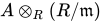
局所環上の例 局所可換環 が与えられたとき 、 - 代数 が Azumaya であるための必要十分条件は、が - 加群 として正の有限ランクを持たず 、代数が 上の中心単純代数である場合です。 したがって、すべての例は 上の中心単純代数から来ています 。
( R 、
メートル
)
{\displaystyle (R,{\mathfrak {m}})}
R
{\displaystyle R}
あ
{\displaystyle A}
あ
{\displaystyle A}
R
{\displaystyle R}
あ
⊗
R
( R
/
メートル
)
{\displaystyle A\otimes _{R}(R/{\mathfrak {m}})}
R
/
メートル
{\displaystyle R/{\mathfrak {m}}}
R
/
メートル
{\displaystyle R/{\mathfrak {m}}}
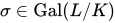
巡回代数 アズマヤ代数のクラスには巡回代数があり、これは体 上のアズマヤ代数のすべての相似クラス 、つまりブラウアー群(以下で定義)のすべての元を生成します。 次数 の 有限巡回ガロア体拡大が与えられると、すべての 生成元と任意の生成元 に対して 、 とも表記される ねじれ多項式環が存在し、これは 次の
元によって生成されます。
け
{\displaystyle K}
Br
( け )
{\displaystyle {\text{Br}}(K)}
ら
/
け
{\displaystyle L/K}
ん
{\displaystyle n}
b ∈
け
∗
{\displaystyle b\in K^{*}}
σ ∈
ギャル
( ら
/
け )
{\displaystyle \sigma \in {\text{Gal}}(L/K)}
ら [ x
]
σ
{\displaystyle L[x]_{\sigma}}
あ ( σ 、 b )
{\displaystyle A(\sigma,b)}
x
{\displaystyle x}
x
ん
= b
{\displaystyle x^{n}=b}
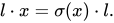
そして次の交換法則が成り立つ。
l ⋅ x = σ ( x ) ⋅ l 。
{\displaystyle l\cdot x=\sigma (x)\cdot l.}
上のベクトル空間として 、は 次のように与えられる乗法を持つ
基底を持ちます。
ら
{\displaystyle L}
ら [ x
]
σ
{\displaystyle L[x]_{\sigma}}
1 、 x 、
x
2
、 … 、
x
ん − 1
{\displaystyle 1,x,x^{2},\ldots ,x^{n-1}}
x
私
⋅
x
じゅう
=
{
x
私 + じゅう
もし
私 + じゅう < ん
x
私 + じゅう − ん
b
もし
私 + じゅう ≥ ん
{\displaystyle x^{i}\cdot x^{j}={\begin{cases}x^{i+j}&{\text{ if }}i+j<n\\x^{i+jn}b&{\text{ if }}i+j\geq n\\\end{cases}}}
幾何学的に整列した多様体 [3] を与えると、商体拡大に関連する巡回代数も存在することに注意する 。
バツ
/
け
{\displaystyle X/K}
フラック
(
バツ
ら
)
/
フラック
( バツ )
{\displaystyle {\text{Frac}}(X_{L})/{\text{Frac}}(X)}
環のブラウアー群 体上では、エタールコホモロジーを 用いたアズマヤ代数のコホモロジー分類が存在する 。実際、 ブラウアー群 と呼ばれるこの群は、環上のアズマヤ代数の 相似類 [1] :3 としても定義することができ 、環は 同型が存在する場合相似である。
R
{\displaystyle R}
あ 、
あ ′
{\displaystyle A,A'}
あ
⊗
R
ま
ん
( R ) ≅
あ ′
⊗
R
ま
メートル
( R )
{\displaystyle A\otimes _{R}M_{n}(R)\cong A'\otimes _{R}M_{m}(R)}
となる。この同値関係は実際には同値関係であり、 、 、 であれば 、 となり、
n
,
m
{\displaystyle n,m}
A
1
∼
A
1
′
{\displaystyle A_{1}\sim A_{1}'}
A
2
∼
A
2
′
{\displaystyle A_{2}\sim A_{2}'}
A
1
⊗
R
A
2
∼
A
1
′
⊗
R
A
2
′
{\displaystyle A_{1}\otimes _{R}A_{2}\sim A_{1}'\otimes _{R}A_{2}'}
[
A
1
]
⊗
[
A
2
]
=
[
A
1
⊗
R
A
2
]
{\displaystyle [A_{1}]\otimes [A_{2}]=[A_{1}\otimes _{R}A_{2}]}
は明確に定義された演算である。これは、そのような同値類の集合上に、 ブラウアー群 と呼ばれる群構造を形成し、 と表記される 。別の定義は、エタールコホモロジー群の捩れ部分群によって与えられる。
Br
(
R
)
{\displaystyle {\text{Br}}(R)}
Br
coh
(
R
)
:=
H
e
t
2
(
Spec
(
R
)
,
G
m
)
tors
{\displaystyle {\text{Br}}_{\text{coh}}(R):={\text{H}}_{et}^{2}({\text{Spec}}(R),\mathbb {G} _{m})_{\text{tors}}}
これはコホモロジー的ブラウアー群 と呼ばれる 。これら 2 つの定義は、が 体のときに一致する。
R
{\displaystyle R}
ガロアコホモロジーを用いたブラウアー群 ガロアコホモロジーを 用いたブラウアー群の同等の定義がもう1つある 。体拡大に対して、 コホモロジー的ブラウアー群は次のように定義される。
E
/
F
{\displaystyle E/F}
Br
coh
(
E
/
F
)
:=
H
Gal
2
(
Gal
(
E
/
F
)
,
E
×
)
{\displaystyle {\text{Br}}^{\text{coh}}(E/F):=H_{\text{Gal}}^{2}({\text{Gal}}(E/F),E^{\times })}
に対するコホモロジー的ブラウアー群は 次のように定義される。
F
{\displaystyle F}
Br
coh
(
F
)
=
colim
E
/
F
H
Gal
2
(
Gal
(
E
/
F
)
,
E
×
)
{\displaystyle {\text{Br}}^{\text{coh}}(F)={\underset {E/F}{\text{colim}}}H_{\text{Gal}}^{2}({\text{Gal}}(E/F),E^{\times })}
ここで、余極限はすべての有限ガロア体拡大に対して取られます。
局所フィールドの計算 p 進数 のような 局所非アルキメデス体上では 、 局所類体理論は アーベル群の同型性を与える: [4] 193ページ
F
{\displaystyle F}
Q
p
{\displaystyle \mathbb {Q} _{p}}
Br
coh
(
F
)
≅
Q
/
Z
.
{\displaystyle {\text{Br}}^{\text{coh}}(F)\cong \mathbb {Q} /\mathbb {Z} .}
これは、アーベル体拡大が与えられた場合、 ガロア群の短い完全列が存在する
ためである。
E
2
/
E
1
/
F
{\displaystyle E_{2}/E_{1}/F}
0
→
Gal
(
E
2
/
E
1
)
→
Gal
(
E
2
/
F
)
→
Gal
(
E
1
/
F
)
→
0
{\displaystyle 0\to {\text{Gal}}(E_{2}/E_{1})\to {\text{Gal}}(E_{2}/F)\to {\text{Gal}}(E_{1}/F)\to 0}
局所類体理論から、次の可換図式が存在する: [5]
H
Gal
2
(
Gal
(
E
2
/
F
)
,
E
1
×
)
→
H
Gal
2
(
Gal
(
E
1
/
F
)
,
E
1
×
)
↓
↓
(
1
[
E
2
:
E
1
]
Z
)
/
Z
→
(
1
[
E
1
:
F
]
Z
)
/
Z
{\displaystyle {\begin{matrix}H_{\text{Gal}}^{2}({\text{Gal}}(E_{2}/F),E_{1}^{\times })&\to &H_{\text{Gal}}^{2}({\text{Gal}}(E_{1}/F),E_{1}^{\times })\\\downarrow &&\downarrow \\\left({\frac {1}{[E_{2}:E_{1}]}}\mathbb {Z} \right)/\mathbb {Z} &\to &\left({\frac {1}{[E_{1}:F]}}\mathbb {Z} \right)/\mathbb {Z} \end{matrix}}}
ここで、垂直マップは同型であり、水平マップは注入です。
ん -フィールドのねじれ クンマーシーケンス [6]があることを思い出してください。
1
→
μ
n
→
G
m
→
⋅
n
G
m
→
1
{\displaystyle 1\to \mu _{n}\to \mathbb {G} _{m}\xrightarrow {\cdot n} \mathbb {G} _{m}\to 1}
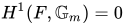
は体 のコホモロジーにおける長完全列を与える 。 ヒルベルトの定理90 が示すように 、関連する短完全列が存在する。
F
{\displaystyle F}
H
1
(
F
,
G
m
)
=
0
{\displaystyle H^{1}(F,\mathbb {G} _{m})=0}
0
→
H
e
t
2
(
F
,
μ
n
)
→
Br
(
F
)
→
⋅
n
Br
(
F
)
→
0
{\displaystyle 0\to H_{et}^{2}(F,\mu _{n})\to {\text{Br}}(F)\xrightarrow {\cdot n} {\text{Br}}(F)\to 0}
係数が1の乗根 である第2エタールコホモロジー群を示すと 、
n
{\displaystyle n}
μ
n
{\displaystyle \mu _{n}}
H
e
t
2
(
F
,
μ
n
)
=
Br
(
F
)
n
-tors
.
{\displaystyle H_{et}^{2}(F,\mu _{n})={\text{Br}}(F)_{n{\text{-tors}}}.}
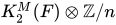
ジェネレーターの ん -体上のブラウアー群の捩れ類 ガロア記号 、 またはノルム留数記号は、 -捩れ ミルナーK理論 群から エタールコホモロジー群 への写像であり 、次のように表される。
n
{\displaystyle n}
K
2
M
(
F
)
⊗
Z
/
n
{\displaystyle K_{2}^{M}(F)\otimes \mathbb {Z} /n}
H
e
t
2
(
F
,
μ
n
⊗
2
)
{\displaystyle H_{et}^{2}(F,\mu _{n}^{\otimes 2})}
R
n
,
F
:
K
2
M
(
F
)
⊗
Z
Z
/
n
Z
→
H
e
t
2
(
F
,
μ
n
⊗
2
)
{\displaystyle R_{n,F}:K_{2}^{M}(F)\otimes _{\mathbb {Z} }\mathbb {Z} /n\mathbb {Z} \to H_{et}^{2}(F,\mu _{n}^{\otimes 2})}
[6] これは、エタールコホモロジーにおけるカップ積とヒルベルトの定理90の同型性の合成から得られる。
χ
n
,
F
:
F
∗
⊗
Z
Z
/
n
→
H
et
1
(
F
,
μ
n
)
{\displaystyle \chi _{n,F}:F^{*}\otimes _{\mathbb {Z} }\mathbb {Z} /n\to H_{\text{et}}^{1}(F,\mu _{n})}
したがって
R
n
,
F
(
{
a
,
b
}
)
=
χ
n
,
F
(
a
)
∪
χ
n
,
F
(
b
)
{\displaystyle R_{n,F}(\{a,b\})=\chi _{n,F}(a)\cup \chi _{n,F}(b)}
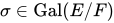
この写像は を介して因数分解され 、 の に対するクラスは 巡回代数 によって表される 。 となる クンマー拡大 に対して、巡回群の 生成元を取り、 を構築します。 ガロアコホモロジー およびエタールコホモロジーを介して、代替的でありながら同等な構成があります。自明な - 加群
の短完全列を考えてみましょう。
H
et
2
(
F
,
μ
n
)
=
Br
(
F
)
n
-tors
{\displaystyle H_{\text{et}}^{2}(F,\mu _{n})={\text{Br}}(F)_{n{\text{-tors}}}}
{
a
,
b
}
{\displaystyle \{a,b\}}
[
A
(
σ
,
b
)
]
{\displaystyle [A(\sigma ,b)]}
E
/
F
{\displaystyle E/F}
E
=
F
(
a
n
)
{\displaystyle E=F({\sqrt[{n}]{a}})}
σ
∈
Gal
(
E
/
F
)
{\displaystyle \sigma \in {\text{Gal}}(E/F)}
[
A
(
σ
,
b
)
]
{\displaystyle [A(\sigma ,b)]}
Gal
(
F
¯
/
F
)
{\displaystyle {\text{Gal}}({\overline {F}}/F)}
0
→
Z
→
Z
→
Z
/
n
→
0
{\displaystyle 0\to \mathbb {Z} \to \mathbb {Z} \to \mathbb {Z} /n\to 0}
長完全列はマップを生成する
H
Gal
1
(
F
,
Z
/
n
)
→
δ
H
Gal
2
(
F
,
Z
)
{\displaystyle H_{\text{Gal}}^{1}(F,\mathbb {Z} /n)\xrightarrow {\delta } H_{\text{Gal}}^{2}(F,\mathbb {Z} )}
ユニークなキャラクター
χ
:
Gal
(
E
/
F
)
→
Z
/
n
{\displaystyle \chi :{\text{Gal}}(E/F)\to \mathbb {Z} /n}
には ユニークなリフトがあります
χ
(
σ
)
=
1
{\displaystyle \chi (\sigma )=1}
χ
¯
:
Gal
(
F
¯
/
F
)
→
Z
/
n
{\displaystyle {\overline {\chi }}:{\text{Gal}}({\overline {F}}/F)\to \mathbb {Z} /n}
そして
δ
(
χ
¯
)
∪
(
b
)
=
[
A
(
σ
,
b
)
]
∈
Br
(
F
)
{\displaystyle \delta ({\overline {\chi }})\cup (b)=[A(\sigma ,b)]\in {\text{Br}}(F)}
クラスは ヒルベルトの定理90マップから来ていることに注意 。すると、原始根が存在するので 、クラスも存在する。
(
b
)
{\displaystyle (b)}
χ
n
,
F
(
b
)
{\displaystyle \chi _{n,F}(b)}
ζ
∈
μ
n
⊂
F
{\displaystyle \zeta \in \mu _{n}\subset F}
δ
(
χ
¯
)
∪
(
b
)
∪
(
ζ
)
∈
H
et
2
(
F
,
μ
n
⊗
2
)
{\displaystyle \delta ({\overline {\chi }})\cup (b)\cup (\zeta )\in H_{\text{et}}^{2}(F,\mu _{n}^{\otimes 2})}
これはまさにクラス であることがわかります。 ノルム留数同型定理 により 、 は同型であり、 の -捩れクラスは 巡回代数 によって生成されます 。
R
n
,
F
(
{
a
,
b
}
)
{\displaystyle R_{n,F}(\{a,b\})}
R
n
,
F
{\displaystyle R_{n,F}}
n
{\displaystyle n}
Br
(
F
)
n
-tors
{\displaystyle {\text{Br}}(F)_{n{\text{-tors}}}}
[
A
(
σ
,
b
)
]
{\displaystyle [A(\sigma ,b)]}
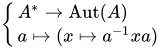
スコーレム・ノイマン定理 アズマヤ代数に関する重要な構造的結果の 1 つは、 スコーレム・ノイマン定理 です。局所可換環 とアズマヤ代数が与えられた場合 、 の唯一の自己同型は 内部です。つまり、次のマップは全射です。
R
{\displaystyle R}
R
→
A
{\displaystyle R\to A}
A
{\displaystyle A}
{
A
∗
→
Aut
(
A
)
a
↦
(
x
↦
a
−
1
x
a
)
{\displaystyle {\begin{cases}A^{*}\to {\text{Aut}}(A)\\a\mapsto (x\mapsto a^{-1}xa)\end{cases}}}
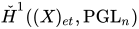
ここで、 は の単位 群 である 。これは、スキーム上のアズマヤ代数の相似類のコホモロジー分類に直接関係するため重要である。特に、アズマヤ代数は、 ある に対して構造群を持ち 、 チェフコホモロジー 群は
A
∗
{\displaystyle A^{*}}
A
.
{\displaystyle A.}
PGL
n
{\displaystyle {\text{PGL}}_{n}}
n
{\displaystyle n}
H
ˇ
1
(
(
X
)
e
t
,
PGL
n
)
{\displaystyle {\check {H}}^{1}((X)_{et},{\text{PGL}}_{n})}
はそのような束のコホモロジー分類を与える。そしてこれは、 正確なシーケンス
H
et
2
(
X
,
G
m
)
{\displaystyle H_{\text{et}}^{2}(X,\mathbb {G} _{m})}
1
→
G
m
→
GL
n
→
PGL
n
→
1
{\displaystyle 1\to \mathbb {G} _{m}\to {\text{GL}}_{n}\to {\text{PGL}}_{n}\to 1}
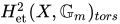
の像は、 ねじれ部分群の部分群であることがわかります 。
H
1
{\displaystyle H^{1}}
H
et
2
(
X
,
G
m
)
t
o
r
s
{\displaystyle H_{\text{et}}^{2}(X,\mathbb {G} _{m})_{tors}}
計画について 構造層 を持つ スキーム X 上のアズマヤ代数は、元のグロタンディークセミナーによれば、行列代数層に局所的にエタール同型である -代数 の層です 。ただし、各行列代数層は正のランクであるという条件を追加する必要があります。この定義により、 上のアズマヤ代数は 層の「ねじれた形式」になります 。ミルンの エタールコホモロジーで は、代わりに、各点での 茎が 上記の意味で
局所環 上のアズマヤ代数である-代数 の 層であるという定義から出発しています。
O
X
{\displaystyle {\mathcal {O}}_{X}}
A
{\displaystyle {\mathcal {A}}}
O
X
{\displaystyle {\mathcal {O}}_{X}}
(
X
,
O
X
)
{\displaystyle (X,{\mathcal {O}}_{X})}
M
n
(
O
X
)
{\displaystyle M_{n}({\mathcal {O}}_{X})}
A
{\displaystyle {\mathcal {A}}}
O
X
{\displaystyle {\mathcal {O}}_{X}}
A
x
{\displaystyle {\mathcal {A}}_{x}}
x
{\displaystyle x}
O
X
,
x
{\displaystyle {\mathcal {O}}_{X,x}}
2つの東谷代数 とが 同値で あるのは、 任意の点において有限の正のランクを持つ
局所自由層 とが 存在する場合である。
A
1
{\displaystyle {\mathcal {A}}_{1}}
A
2
{\displaystyle {\mathcal {A}}_{2}}
E
1
{\displaystyle {\mathcal {E}}_{1}}
E
2
{\displaystyle {\mathcal {E}}_{2}}
A
1
⊗
E
n
d
O
X
(
E
1
)
≃
A
2
⊗
E
n
d
O
X
(
E
2
)
,
{\displaystyle A_{1}\otimes \mathrm {End} _{{\mathcal {O}}_{X}}({\mathcal {E}}_{1})\simeq A_{2}\otimes \mathrm {End} _{{\mathcal {O}}_{X}}({\mathcal {E}}_{2}),}
[1] : 6 ここで は の自己準同型層です。 の ブラウアー群(体の ブラウアー群 の類似体) は、東谷代数の同値類の集合です。群演算はテンソル積で与えられ、逆演算は反対代数で与えられます。これは として定義される コホモロジー ブラウアー群 とは異なることに注意してください 。
E
n
d
O
X
(
E
i
)
{\displaystyle \mathrm {End} _{{\mathcal {O}}_{X}}({\mathcal {E}}_{i})}
E
i
{\displaystyle {\mathcal {E}}_{i}}
B
(
X
)
{\displaystyle B(X)}
X
{\displaystyle X}
H
et
2
(
X
,
G
m
)
{\displaystyle H_{\text{et}}^{2}(X,\mathbb {G} _{m})}
仕様上の例( ず [1/ ん ]) 体上の四元数代数の構成は、 非可換代 数
を考えることによってグローバル化できる。
Spec
(
Z
[
1
/
n
]
)
{\displaystyle {\text{Spec}}(\mathbb {Z} [1/n])}
Z
[
1
/
n
]
{\displaystyle \mathbb {Z} [1/n]}
A
a
,
b
=
Z
[
1
/
n
]
⟨
i
,
j
,
k
⟩
i
2
−
a
,
j
2
−
b
,
i
j
−
k
,
j
i
+
k
{\displaystyle A_{a,b}={\frac {\mathbb {Z} [1/n]\langle i,j,k\rangle }{i^{2}-a,j^{2}-b,ij-k,ji+k}}}
すると、-代数の層として 、 アズマヤ代数の構造を持つ。開アフィン集合に制限する理由は 、四元数代数が点上の除算代数であり 、 ヒルベルト記号
O
X
{\displaystyle {\mathcal {O}}_{X}}
A
a
,
b
{\displaystyle {\mathcal {A}}_{a,b}}
Spec
(
Z
[
1
/
n
]
)
↪
Spec
(
Z
)
{\displaystyle {\text{Spec}}(\mathbb {Z} [1/n])\hookrightarrow {\text{Spec}}(\mathbb {Z} )}
(
p
)
{\displaystyle (p)}
(
a
,
b
)
p
=
1
{\displaystyle (a,b)_{p}=1}
これは、有限個の素数を除いてすべてに当てはまります。
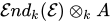
例終了 ポ ん アズマヤ代数上は、 体上の アズマヤ代数に対して と同様に構成できる 。例えば、の自己準同型層は 行列層である。
P
k
n
{\displaystyle \mathbb {P} _{k}^{n}}
E
n
d
k
(
E
)
⊗
k
A
{\displaystyle {\mathcal {End}}_{k}({\mathcal {E}})\otimes _{k}A}
A
{\displaystyle A}
k
{\displaystyle k}
O
(
a
)
⊕
O
(
b
)
{\displaystyle {\mathcal {O}}(a)\oplus {\mathcal {O}}(b)}
E
n
d
k
(
O
(
a
)
⊕
O
(
b
)
)
=
(
O
O
(
b
−
a
)
O
(
a
−
b
)
O
)
{\displaystyle {\mathcal {End}}_{k}({\mathcal {O}}(a)\oplus {\mathcal {O}}(b))={\begin{pmatrix}{\mathcal {O}}&{\mathcal {O}}(b-a)\\{\mathcal {O}}(a-b)&{\mathcal {O}}\end{pmatrix}}}
したがって、 上のアズマヤ代数は 、四元数代数などの
上の アズマヤ代数でテンソル化されたこの層から構築できます。
P
k
n
{\displaystyle \mathbb {P} _{k}^{n}}
A
{\displaystyle A}
k
{\displaystyle k}
アプリケーション ユーリ・マニン の研究に続いて、 ディオファントス幾何学 における東谷代数の重要な応用がありました 。 ハッセ原理 に対する マニンの障害は 、ブラウアー群のスキームを使用して定義されます。
参照
参考文献
^ abc ミルン、ジェームス S. (1980)。エタールのコホモロジー (PDF) 。ニュージャージー州プリンストン:プリンストン大学出版局。 ISBN 0-691-08238-3 . OCLC 5028959. 2020年6月21日時点のオリジナル (PDF) よりアーカイブ。 ^ Borceux, Francis; Vitale, Enrico (2002). 「Azumaya カテゴリ」 (PDF) . 応用カテゴリ構造 . 10 : 449–467. ^ つまり、その基底体の代数閉包まで拡張すると整多様体となる。 ^ セール、ジャン・ピエール。 (1979年)。ローカルフィールド。ニューヨーク州ニューヨーク: スプリンガー ニューヨーク。 ISBN 978-1-4757-5673-9 . OCLC 859586064. ^ 「コホモロジー類体理論に関する講義」 (PDF) 。 2020年6月22日時点のオリジナルより アーカイブ (PDF) 。 ^ ab Srinivas, V. (1994). 「8. メルクリェフ-ススリン定理」. 代数的 K 理論 (第 2 版). ボストン、マサチューセッツ州: Birkhäuser Boston. pp. 145–193. ISBN 978-0-8176-4739-1 . OCLC 853264222.
ブラウアー群と東谷代数 ミルン、ジョン。エタールコホモロジー。第 IV 章 マックス・アルバート・クヌース;オジャングレン、マヌエル (1974)、 Theorie de la descente et algebres d'Azumaya 、Lecture Notes in Mathematics、vol. 389、ベルリン、ニューヨーク: Springer-Verlag 、 doi :10.1007/BFb0057799、 MR 0417149、 Zbl 0284.13002 「Azumaya 代数の明示的な例」に関する Mathoverflow スレッド 除算代数 Knus、Max-Albert (1991)、 リング上の二次形式とエルミート形式 、Grundlehren der Mathematischen Wissenschaften、vol. 294、ベルリンなど: Springer-Verlag 、 ISBN 3-540-52117-8 、 ZBL 0756.11008 Saltman, David J. (1999)。 除算代数の講義 。 数学地域会議シリーズ。第 94 巻。プロビデンス、ロードアイランド州: アメリカ数学協会 。ISBN 0-8218-0979-2 .ZBL0934.16013 .





![{\displaystyle L[x]_{\sigma}}](https://wikimedia.org/api/rest_v1/media/math/render/svg/215e7b221f1476875f9be105760062386924a7d7)












![{\displaystyle [A_{1}]\otimes [A_{2}]=[A_{1}\otimes _{R}A_{2}]}](https://wikimedia.org/api/rest_v1/media/math/render/svg/241784562a9a8ca3ef00bb05014fba7ae8f2a9bd)










![{\displaystyle {\begin{matrix}H_{\text{Gal}}^{2}({\text{Gal}}(E_{2}/F),E_{1}^{\times })&\to &H_{\text{Gal}}^{2}({\text{Gal}}(E_{1}/F),E_{1}^{\times })\\\downarrow &&\downarrow \\\left({\frac {1}{[E_{2}:E_{1}]}}\mathbb {Z} \right)/\mathbb {Z} &\to &\left({\frac {1}{[E_{1}:F]}}\mathbb {Z} \right)/\mathbb {Z} \end{matrix}}}](https://wikimedia.org/api/rest_v1/media/math/render/svg/da101032e8171d1844c95f2172d96d66d153523d)










![{\displaystyle [A(\sigma ,b)]}](https://wikimedia.org/api/rest_v1/media/math/render/svg/8329d89e02ad0acd38fad1f93a01481a91a9e345)
![{\displaystyle E=F({\sqrt[{n}]{a}})}](https://wikimedia.org/api/rest_v1/media/math/render/svg/a9ad2a7cbf89a40df2029838d54e927b7065cf44)






![{\displaystyle \delta ({\overline {\chi}})\cup (b)=[A(\sigma ,b)]\in {\text{Br}}(F)}](https://wikimedia.org/api/rest_v1/media/math/render/svg/5145acdeb6c1089b662460c1206ae4b2dee1817c)















![{\displaystyle {\text{Spec}}(\mathbb {Z} [1/n])}](https://wikimedia.org/api/rest_v1/media/math/render/svg/66f967aac8e21c47d6d2089dc1c74c4305a63b59)
![{\displaystyle \mathbb {Z} [1/n]}](https://wikimedia.org/api/rest_v1/media/math/render/svg/c76756ee50c9bbb59867be3d1709fc4ead722b47)
![{\displaystyle A_{a,b}={\frac {\mathbb {Z} [1/n]\langle i,j,k\rangle }{i^{2}-a,j^{2}-b 、ij-k、ji+k}}}](https://wikimedia.org/api/rest_v1/media/math/render/svg/1bac55729dab8602918b660053e63bdaaed7ee96)

![{\displaystyle {\text{Spec}}(\mathbb {Z} [1/n])\hookrightarrow {\text{Spec}}(\mathbb {Z} )}](https://wikimedia.org/api/rest_v1/media/math/render/svg/a1e4e1dfeb8fe41574548f6873f2172f96a5a499)