三角関数を含む積分の変数変換
積分学 において 、 接線半角置換は、 積分 を評価するために用いられる 変数変換 であり 、 と設定することにより、 の 三角関数 の 有理 関数を の 通常の有理関数に変換する。これは、 角度測度 によってパラメータ化された 単位円 の実数 直線 上への 1次元 立体射影 である。一般的な [1] 変換式は次の通りである。
x
{\textstyle x}
t
{\textstyle t}
t
=
tan
x
2
{\textstyle t=\tan {\tfrac {x}{2}}}
∫
f
(
sin
x
,
cos
x
)
d
x
=
∫
f
(
2
t
1
+
t
2
,
1
−
t
2
1
+
t
2
)
2
d
t
1
+
t
2
.
{\displaystyle \int f(\sin x,\cos x)\,dx=\int f{\left({\frac {2t}{1+t^{2}}},{\frac {1-t^{2}}{1+t^{2}}}\right)}{\frac {2\,dt}{1+t^{2}}}.}
半角の正接は 球面三角法 において重要であり、17世紀には半正接または半正接として知られていました。 [2] レオンハルト・オイラーは 1768年の積分学の教科書 で これを積分の評価に使用し 、 [3] アドリアン ・マリー・ルジャンドルは 1817年に一般的な方法を説明しました 。[4]
∫
d
x
/
(
a
+
b
cos
x
)
{\textstyle \int dx/(a+b\cos x)}
この置換法は、19世紀後半からほとんどの積分学の教科書で説明されているが、通常は特別な名前は付けられていない。 [5]ロシアでは 普遍三角置換法 として知られており 、 [6] 半接線置換法 や 半角置換法 などの別名でも知られている。ワイエルシュ トラス置換法 と誤って呼ばれることもある 。 [7] マイケル・スピヴァクは これを「世界で最もずる賢い置換法」と呼んだ。 [8]
代替 接線半角置換は、角度を線の傾きに関連付けます。 新しい変数を導入すると、正弦と余弦は の 有理関数 として表すことができ 、 は と の有理関数の 積として 次のように表すことができます。
t
=
tan
x
2
,
{\textstyle t=\tan {\tfrac {x}{2}},}
t
,
{\displaystyle t,}
d
x
{\displaystyle dx}
d
t
{\displaystyle dt}
t
,
{\displaystyle t,}
sin
x
=
2
t
1
+
t
2
,
cos
x
=
1
−
t
2
1
+
t
2
,
and
d
x
=
2
1
+
t
2
d
t
.
{\displaystyle \sin x={\frac {2t}{1+t^{2}}},\quad \cos x={\frac {1-t^{2}}{1+t^{2}}},\quad {\text{and}}\quad dx={\frac {2}{1+t^{2}}}\,dt.}
tan x 、 cot x 、 sec x 、 csc x についても同様の式を書くことができます 。
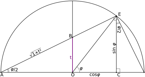
導出 二倍角の公式 と ピタゴラスの定理 を用いて 分母を1にすると、次の式 が得られます。
sin
x
=
2
sin
x
2
cos
x
2
{\displaystyle \sin x=2\sin {\tfrac {x}{2}}\cos {\tfrac {x}{2}}}
cos
x
=
cos
2
x
2
−
sin
2
x
2
{\displaystyle \cos x=\cos ^{2}{\tfrac {x}{2}}-\sin ^{2}{\tfrac {x}{2}}}
1
=
cos
2
x
2
+
sin
2
x
2
{\displaystyle 1=\cos ^{2}{\tfrac {x}{2}}+\sin ^{2}{\tfrac {x}{2}}}
sin
x
=
2
sin
x
2
cos
x
2
cos
2
x
2
+
sin
2
x
2
=
2
tan
x
2
1
+
tan
2
x
2
=
2
t
1
+
t
2
,
cos
x
=
cos
2
x
2
−
sin
2
x
2
cos
2
x
2
+
sin
2
x
2
=
1
−
tan
2
x
2
1
+
tan
2
x
2
=
1
−
t
2
1
+
t
2
.
{\displaystyle {\begin{aligned}\sin x&={\frac {2\sin {\tfrac {x}{2}}\,\cos {\tfrac {x}{2}}}{\cos ^{2}{\tfrac {x}{2}}+\sin ^{2}{\tfrac {x}{2}}}}={\frac {2\tan {\tfrac {x}{2}}}{1+\tan ^{2}{\tfrac {x}{2}}}}={\frac {2t}{1+t^{2}}},\\[18mu]\cos x&={\frac {\cos ^{2}{\tfrac {x}{2}}-\sin ^{2}{\tfrac {x}{2}}}{\cos ^{2}{\tfrac {x}{2}}+\sin ^{2}{\tfrac {x}{2}}}}={\frac {1-\tan ^{2}{\tfrac {x}{2}}}{1+\tan ^{2}{\tfrac {x}{2}}}}={\frac {1-t^{2}}{1+t^{2}}}.\end{aligned}}}
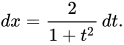
最後に、 なので 、 微分規則 は
t
=
tan
x
2
{\textstyle t=\tan {\tfrac {x}{2}}}
d
t
=
1
2
(
1
+
tan
2
x
2
)
d
x
=
1
+
t
2
2
d
x
,
{\displaystyle dt={\tfrac {1}{2}}\left(1+\tan ^{2}{\tfrac {x}{2}}\right)dx={\frac {1+t^{2}}{2}}\,dx,}
そしてこうして
d
x
=
2
1
+
t
2
d
t
.
{\displaystyle dx={\frac {2}{1+t^{2}}}\,dt.}
例
コセカントの不定積分
∫
csc
x
d
x
=
∫
d
x
sin
x
=
∫
(
1
+
t
2
2
t
)
(
2
1
+
t
2
)
d
t
t
=
tan
x
2
=
∫
d
t
t
=
ln
|
t
|
+
C
=
ln
|
tan
x
2
|
+
C
.
{\displaystyle {\begin{aligned}\int \csc x\,dx&=\int {\frac {dx}{\sin x}}\\[6pt]&=\int \left({\frac {1+t^{2}}{2t}}\right)\left({\frac {2}{1+t^{2}}}\right)dt&&t=\tan {\tfrac {x}{2}}\\[6pt]&=\int {\frac {dt}{t}}\\[6pt]&=\ln |t|+C\\[6pt]&=\ln \left|\tan {\tfrac {x}{2}}\right|+C.\end{aligned}}}
上記の結果は、分子と分母に を掛けて 代入を行うことで、コセカント積分を評価する標準的な方法を使用して確認できます 。
csc
x
−
cot
x
{\textstyle \csc x-\cot x}
u
=
csc
x
−
cot
x
,
{\textstyle u=\csc x-\cot x,}
d
u
=
(
−
csc
x
cot
x
+
csc
2
x
)
d
x
{\textstyle du=\left(-\csc x\cot x+\csc ^{2}x\right)\,dx}
∫
csc
x
d
x
=
∫
csc
x
(
csc
x
−
cot
x
)
csc
x
−
cot
x
d
x
=
∫
(
csc
2
x
−
csc
x
cot
x
)
d
x
csc
x
−
cot
x
u
=
csc
x
−
cot
x
=
∫
d
u
u
=
ln
|
u
|
+
C
=
ln
|
csc
x
−
cot
x
|
+
C
.
{\displaystyle {\begin{aligned}\int \csc x\,dx&=\int {\frac {\csc x(\csc x-\cot x)}{\csc x-\cot x}}\,dx\\[6pt]&=\int {\frac {\left(\csc ^{2}x-\csc x\cot x\right)\,dx}{\csc x-\cot x}}\qquad u=\csc x-\cot x\\[6pt]&=\int {\frac {du}{u}}\\[6pt]&=\ln |u|+C\\[6pt]&=\ln \left|\csc x-\cot x\right|+C.\end{aligned}}}
これら2つの答えは同じです。
csc
x
−
cot
x
=
tan
x
2
:
{\textstyle \csc x-\cot x=\tan {\tfrac {x}{2}}\colon }
csc
x
−
cot
x
=
1
sin
x
−
cos
x
sin
x
=
1
+
t
2
2
t
−
1
−
t
2
1
+
t
2
1
+
t
2
2
t
t
=
tan
x
2
=
2
t
2
2
t
=
t
=
tan
x
2
{\displaystyle {\begin{aligned}\csc x-\cot x&={\frac {1}{\sin x}}-{\frac {\cos x}{\sin x}}\\[6pt]&={\frac {1+t^{2}}{2t}}-{\frac {1-t^{2}}{1+t^{2}}}{\frac {1+t^{2}}{2t}}\qquad \qquad t=\tan {\tfrac {x}{2}}\\[6pt]&={\frac {2t^{2}}{2t}}=t\\[6pt]&=\tan {\tfrac {x}{2}}\end{aligned}}}
正 割積分も 同様の方法で評価できます。
定積分
∫
0
2
π
d
x
2
+
cos
x
=
∫
0
π
d
x
2
+
cos
x
+
∫
π
2
π
d
x
2
+
cos
x
=
∫
0
∞
2
d
t
3
+
t
2
+
∫
−
∞
0
2
d
t
3
+
t
2
t
=
tan
x
2
=
∫
−
∞
∞
2
d
t
3
+
t
2
=
2
3
∫
−
∞
∞
d
u
1
+
u
2
t
=
u
3
=
2
π
3
.
{\displaystyle {\begin{aligned}\int _{0}^{2\pi }{\frac {dx}{2+\cos x}}&=\int _{0}^{\pi }{\frac {dx}{2+\cos x}}+\int _{\pi }^{2\pi }{\frac {dx}{2+\cos x}}\\[6pt]&=\int _{0}^{\infty }{\frac {2\,dt}{3+t^{2}}}+\int _{-\infty }^{0}{\frac {2\,dt}{3+t^{2}}}&t&=\tan {\tfrac {x}{2}}\\[6pt]&=\int _{-\infty }^{\infty }{\frac {2\,dt}{3+t^{2}}}\\[6pt]&={\frac {2}{\sqrt {3}}}\int _{-\infty }^{\infty }{\frac {du}{1+u^{2}}}&t&=u{\sqrt {3}}\\[6pt]&={\frac {2\pi }{\sqrt {3}}}.\end{aligned}}}
最初の行では、 積分 の 両方の限界を単純に代入する ことはできません 。における の 特異点 (この場合は、 垂直漸近線 ) を考慮する必要があります。 または、まず不定積分を評価し、次に境界値を適用します。
対称性により、
これは前の回答と同じです。
t
=
0
{\textstyle t=0}
t
=
tan
x
2
{\textstyle t=\tan {\tfrac {x}{2}}}
x
=
π
{\textstyle x=\pi }
∫
d
x
2
+
cos
x
=
∫
1
2
+
1
−
t
2
1
+
t
2
2
d
t
t
2
+
1
t
=
tan
x
2
=
∫
2
d
t
2
(
t
2
+
1
)
+
(
1
−
t
2
)
=
∫
2
d
t
t
2
+
3
=
2
3
∫
d
t
(
t
/
3
)
2
+
1
u
=
t
/
3
=
2
3
∫
d
u
u
2
+
1
tan
θ
=
u
=
2
3
∫
cos
2
θ
sec
2
θ
d
θ
=
2
3
∫
d
θ
=
2
3
θ
+
C
=
2
3
arctan
(
t
3
)
+
C
=
2
3
arctan
(
tan
x
2
3
)
+
C
.
{\displaystyle {\begin{aligned}\int {\frac {dx}{2+\cos x}}&=\int {\frac {1}{2+{\frac {1-t^{2}}{1+t^{2}}}}}{\frac {2\,dt}{t^{2}+1}}&&t=\tan {\tfrac {x}{2}}\\[6pt]&=\int {\frac {2\,dt}{2(t^{2}+1)+(1-t^{2})}}=\int {\frac {2\,dt}{t^{2}+3}}\\[6pt]&={\frac {2}{3}}\int {\frac {dt}{{\bigl (}t{\big /}{\sqrt {3}}{\bigr )}^{2}+1}}&&u=t{\big /}{\sqrt {3}}\\[6pt]&={\frac {2}{\sqrt {3}}}\int {\frac {du}{u^{2}+1}}&&\tan \theta =u\\[6pt]&={\frac {2}{\sqrt {3}}}\int \cos ^{2}\theta \sec ^{2}\theta \,d\theta ={\frac {2}{\sqrt {3}}}\int d\theta \\[6pt]&={\frac {2}{\sqrt {3}}}\theta +C={\frac {2}{\sqrt {3}}}\arctan \left({\frac {t}{\sqrt {3}}}\right)+C\\[6pt]&={\frac {2}{\sqrt {3}}}\arctan \left({\frac {\tan {\tfrac {x}{2}}}{\sqrt {3}}}\right)+C.\end{aligned}}}
∫
0
2
π
d
x
2
+
cos
x
=
2
∫
0
π
d
x
2
+
cos
x
=
lim
b
→
π
4
3
arctan
(
tan
x
2
3
)
|
0
b
=
4
3
[
lim
b
→
π
arctan
(
tan
b
2
3
)
−
arctan
(
0
)
]
=
4
3
(
π
2
−
0
)
=
2
π
3
,
{\displaystyle {\begin{aligned}\int _{0}^{2\pi }{\frac {dx}{2+\cos x}}&=2\int _{0}^{\pi }{\frac {dx}{2+\cos x}}=\lim _{b\rightarrow \pi }{\frac {4}{\sqrt {3}}}\arctan \left({\frac {\tan {\tfrac {x}{2}}}{\sqrt {3}}}\right){\Biggl |}_{0}^{b}\\[6pt]&={\frac {4}{\sqrt {3}}}{\Biggl [}\lim _{b\rightarrow \pi }\arctan \left({\frac {\tan {\tfrac {b}{2}}}{\sqrt {3}}}\right)-\arctan(0){\Biggl ]}={\frac {4}{\sqrt {3}}}\left({\frac {\pi }{2}}-0\right)={\frac {2\pi }{\sqrt {3}}},\end{aligned}}}
3番目の例: 正弦と余弦の両方
∫
d
x
a
cos
x
+
b
sin
x
+
c
=
∫
2
d
t
a
(
1
−
t
2
)
+
2
b
t
+
c
(
t
2
+
1
)
=
∫
2
d
t
(
c
−
a
)
t
2
+
2
b
t
+
a
+
c
=
2
c
2
−
(
a
2
+
b
2
)
arctan
(
(
c
−
a
)
tan
x
2
+
b
c
2
−
(
a
2
+
b
2
)
)
+
C
{\displaystyle {\begin{aligned}\int {\frac {dx}{a\cos x+b\sin x+c}}&=\int {\frac {2\,dt}{a(1-t^{2})+2bt+c(t^{2}+1)}}\\[6pt]&=\int {\frac {2\,dt}{(c-a)t^{2}+2bt+a+c}}\\[6pt]&={\frac {2}{\sqrt {c^{2}-(a^{2}+b^{2})}}}\arctan \left({\frac {(c-a)\tan {\tfrac {x}{2}}+b}{\sqrt {c^{2}-(a^{2}+b^{2})}}}\right)+C\end{aligned}}}
もし
c
2
−
(
a
2
+
b
2
)
>
0.
{\textstyle c^{2}-(a^{2}+b^{2})>0.}
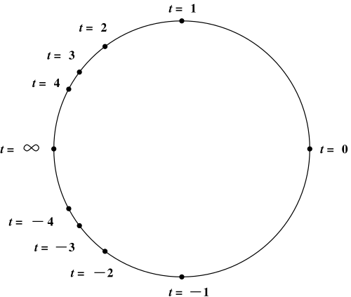
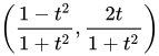
幾何学 接線半角置換は、 (0, 0) を中心とする 単位円 をパラメータ化します。+∞ と −∞ の代わりに、実数の直線の両端に 1 つの ∞ だけがあります。これは、有理関数や三角関数を扱うときによく適切です。(これは 直線の 1 点コンパクト化です。) x が変化すると 、点(cos x 、sin x )は(0、0)を中心とする
単位円 の周りを繰り返し回ります。点
(
1
−
t
2
1
+
t
2
,
2
t
1
+
t
2
)
{\displaystyle \left({\frac {1-t^{2}}{1+t^{2}}},{\frac {2t}{1+t^{2}}}\right)}
t が −∞ から +∞ に向かうとき、点は円を一周するだけで 、点 (−1, 0) に到達することはありません。点 (−1, 0) は、 t が±∞ に向かうにつれて極限に近づきます。t が −∞ から −1 に向かうとき、 t によって決まる点は、 (−1, 0) から (0, −1) まで、第 3 象限の円の部分を通過します 。t が −1 から 0 に向かうとき、点は (0, −1) から (1, 0) まで、第 4 象限の円の部分に従います。t が 0 から 1 に向かうとき 、 点は (1, 0) から (0, 1) まで、第 1 象限の円の部分に従います。最後に、 t が 1 から +∞ に向かうとき、点は (0, 1) から (−1, 0) まで、第 2 象限の円の部分に従います。
ここで、別の幾何学的観点を示します。単位円を描き、 点 Pを (-1, 0)とします。P を 通る直線 (垂直線を除く) はその傾きによって決まります。さらに、各直線 (垂直線を除く) は単位円とちょうど 2 点で交差し、そのうちの 1 つが P です。これにより、単位円上の点から傾きへの関数が決まります。三角関数は、角度から単位円上の点への関数を決定し、これら 2 つの関数を組み合わせると、角度から傾きへの関数が得られます。
双曲線関数 三角関数と双曲関数に共通する他の性質と同様に、 双曲恒等式 を使用して同様の置換形式を構築することができます 。
t
=
tanh
x
2
{\textstyle t=\tanh {\tfrac {x}{2}}}
sinh
x
=
2
t
1
−
t
2
,
cosh
x
=
1
+
t
2
1
−
t
2
,
and
d
x
=
2
1
−
t
2
d
t
.
{\displaystyle \sinh x={\frac {2t}{1-t^{2}}},\quad \cosh x={\frac {1+t^{2}}{1-t^{2}}},\quad {\text{and}}\quad dx={\frac {2}{1-t^{2}}}\,dt.}
同様の式は、 tanh x 、 coth x 、 sech x 、 csch x についても書くことができます 。幾何学的には、この変数変換は、双曲面の ポアンカレ円板モデルに類似した、 双曲 直線の実区間への 1 次元立体投影です 。
代替案 三角関数を積分する方法は他にもあります。たとえば、オイラーの公式 を使用して、三角関数を e ix と e − ix で書き直すと便利です 。
参照
数学ポータル
さらに読む クーラント、リチャード (1937) [1934]。 「1.4.6. その他の関数のクラスの積分 §1–3」 。 微分積分学 。第 1 巻。ブラック & サン。pp. 234–237。 エドワーズ、ジョセフ (1921)。「§1.6.193」。 積分学に関する論文 。第 1 巻。マクミラン。pp. 187–188。 ハーディ、ゴッドフリー・ハロルド (1905)。「VI. 超越関数」。 単一変数関数の積分 。ケンブリッジ。pp. 42–51。 第2版 1916年、52~62ページ チャールズ・エルミート (1873年)。 「Integration des fonctions transdentes」[超越機能の統合]。 Cours d'analyse de l'école Polytechnique (フランス語)。 Vol. 1. ゴーティエ・ヴィラール。 320–380ページ。 Stewart, Seán M. (2017)。「14. 接線半角置換」。 積分方法。 ケンブリッジ 。pp. 178–187。doi : 10.1017 /9781108291507.015。ISBN 978-1-108-41881-2 。
注釈と参考文献
^ 他の三角関数は正弦と余弦で表すことができます。 ^ グンター、エドマンド(1673)[1624]。エドマンド・グンターの著作。フランシス・エグルスフィールド。 73ページ ^ オイラー、レオンハルト (1768)。 「§1.1.5.261 問題 29」 (PDF) 。 Institutiones calculiintegris [ 積分微積分の基礎 ] (ラテン語)。 Vol. I. Impensis Academiae Imperialis Scientiarum。 148~150ページ。 E 342、イアン・ブルース訳。
Lobatto、Rehuel (1832) も参照してください。 「19. Note sur l'intégration de la fonction ∂z / (a + b cos z)」。 クレルの日記 (フランス語)。 9 : 259–260。 ^ ルジャンドル、アドリアン=マリー (1817)。 Exercices de calcul intégral [ 積分計算の演習 ] (フランス語)。 Vol. 2. 配達員。 245~246ページ。 ^ 例えば、時系列順に並べると、
チャールズ・エルミート (1873年)。 Cours d'analyse de l'école Polytechnique (フランス語)。 Vol. 1. ゴーティエ・ヴィラール。 p. 320。 ジョンソン、ウィリアム・ウールジー (1883)。積分学の初等論文。マクミラン。52ページ。 ピカール、エミール (1901) [1891]。 Traité d'analyse (フランス語)。 Vol. 1 (2e 版)。ゴーティエ・ヴィラール。 p. 77. グルサ、エドゥアール (1904) [1902]。数学解析学講座。第 1 巻。ヘドリック、アール レイモンド訳。ギン。pp. 236ff。 ウィルソン、エドウィン・ビッドウェル (1911)。高度な微積分。ギン。 p. 21. エドワーズ、ジョセフ (1921)。積分学に関する論文。第1巻。マクミラン。pp. 187–188。 クーラント、リチャード (1937)[1930]。微分積分学。第1巻。マクシェーン、EJ(第2版)訳。ブラック&サン社。pp.234-238。 ピーターソン、サーマンS.(1950)。 微積分学の要素 。ハーパー&ブラザーズ。pp.201-202。 アポストル、トム・M. (1967) [1961]. 微積分 . 第1巻 (第2版). ゼロックス. pp. 264–265. ラーソン、ロン ; ホステラー、ロバート P.; エドワーズ、ブルース H. (1998) [1978]. 一変数微分積分学 (第 6 版). ホートン ミフリン. p. 520. ISBN 9780395885789 。 ジョン・ロガウスキー (2011) [2008]。 微積分学: 初期の超越論 (第 2 版)。マクミラン。 p. 435.ISBN 9781429231848 。 ^ ピスクノフ、ニコライ (1969年)。微分積分学。Mir。p.379。
ザイツェフ、VV;リシコフ、VV。ミシガン州スカナビ (1978 年)。 初等数学: 復習コース 。 Ėlementarnai͡a matematika.英語。ミル。 p. 388. ^
1966年に ウィリアム・エーベルラインは、 この置き換えを カール・ワイエル シュトラス(1815-1897)によるものとした。
Eberlein, William Frederick (1966). 「循環関数」. Mathematics Magazine . 39 (4): 197–201. doi :10.1080/0025570X.1966.11975715. JSTOR 2688079. (式 (3) [ ],
x
=
cos
θ
{\displaystyle x=\cos \theta }
(4) [ ],
y
=
sin
θ
{\displaystyle y=\sin \theta }
(5) [ ]
t
=
tan
θ
2
{\displaystyle t=\tan {\tfrac {\theta }{2}}}
は、もちろん、ワイエルシュトラスが正弦、余弦の有理関数を積分するために導入した、よく知られた半角置換です。)
20年後、 ジェームズ・スチュワートは、 1987年に最初に出版された人気の微積分教科書の中で、この置換について論じた際にワイエルシュトラスに言及しました。
スチュワート、ジェームズ (1987)。 「§7.5 代入の合理化」 。 微積分 。ブルックス/コール。p. 431。ISBN 9780534066901 ドイツの数学者カール・ワイエルシュトラス(1815–1897)は、 t = tan( x /2) の置換により、 sin x と cos x の任意の有理関数が 通常の有理関数に変換されることに気づきました。
後の著者はスチュワートを引用して、これをワイエルシュトラスの置換 と呼ぶことがあり 、例えば次の通りである。
Jeffrey, David J.; Rich, Albert D. (1994). 「誤った不連続性を回避する三角関数積分の評価」. Transactions on Mathematical Software . 20 (1): 124–135. doi : 10.1145/174603.174409 . S2CID 13891212. ジャン=ピエール・メルレ(2004年)。「三角関数の歴史に関するノート」 (PDF) 。マルコ・チェッカレッリ(編)『 機械とメカニズムの歴史に関する国際シンポジウム』 。クルーワー。pp. 195~200。doi : 10.1007 /1-4020-2204-2_16。ISBN 978-1-4020-2203-6 。 Weisstein, Eric W. (2011). 「Weierstrass Substitution」. MathWorld . 2020年4月1日 閲覧 。
エーベルラインもスチュワートも、ワイエルシュトラスに帰属する証拠を提示していない。ワイエルシュトラスの 『数学全集』 には、1875年の講義で、ワイエルシュトラスは、 次の置換によって 形式の積分を解くというアイデアを カール・ガウス(1818)に帰している。
∫
d
ψ
H
(
sin
ψ
,
cos
ψ
)
/
G
(
sin
ψ
,
cos
ψ
)
{\textstyle \int d\psi \,H(\sin \psi ,\cos \psi ){\big /}{\sqrt {G(\sin \psi ,\cos \psi )}}}
t
=
−
cot
(
ψ
/
2
)
.
{\textstyle t=-\cot(\psi /2).}
ヴァイエルシュトラス、カール (1915) [1875]。 「8. Bestimmung des Integrals ...」。 Mathematische Werke von Karl Weierstrass (ドイツ語)。 Vol. 6. メイヤーとミュラー。 89–99ページ。
^ スピヴァック、マイケル (1967)。「第9章、問題9~10」。 微積分学 。ベンジャミン。pp.325~326。
外部リンク











![{\displaystyle {\begin{aligned}\sin x&={\frac {2\sin {\tfrac {x}{2}}\,\cos {\tfrac {x}{2}}}{\cos ^{2}{\tfrac {x}{2}}+\sin ^{2}{\tfrac {x}{2}}}}={\frac {2\tan {\tfrac {x}{2}}}{1+\tan ^{2}{\tfrac {x}{2}}}}={\frac {2t}{1+t^{2}}},\\[18mu]\cos x&={\frac {\cos ^{2}{\tfrac {x}{2}}-\sin ^{2}{\tfrac {x}{2}}}{\cos ^{2}{\tfrac {x}{2}}+\sin ^{2}{\tfrac {x}{2}}}}={\frac {1-\tan ^{2}{\tfrac {x}{2}}}{1+\tan ^{2}{\tfrac {x}{2}}}}={\frac {1-t^{2}}{1+t^{2}}}.\end{aligned}}}](https://wikimedia.org/api/rest_v1/media/math/render/svg/b0e0db3590824f5019d21786ee97ec792c129906)

![{\displaystyle {\begin{aligned}\int \csc x\,dx&=\int {\frac {dx}{\sin x}}\\[6pt]&=\int \left({\frac {1+t^{2}}{2t}}\right)\left({\frac {2}{1+t^{2}}}\right)dt&&t=\tan {\tfrac {x}{2}}\\[6pt]&=\int {\frac {dt}{t}}\\[6pt]&=\ln |t|+C\\[6pt]&=\ln \left|\tan {\tfrac {x}{2}}\right|+C.\end{aligned}}}](https://wikimedia.org/api/rest_v1/media/math/render/svg/3f619d6c96c3b1dc3e3fd982f2085a01b72147a2)



![{\displaystyle {\begin{aligned}\int \csc x\,dx&=\int {\frac {\csc x(\csc x-\cot x)}{\csc x-\cot x}}\,dx\\[6pt]&=\int {\frac {\left(\csc ^{2}x-\csc x\cot x\right)\,dx}{\csc x-\cot x}}\qquad u=\csc x-\cot x\\[6pt]&=\int {\frac {du}{u}}\\[6pt]&=\ln |u|+C\\[6pt]&=\ln \left|\csc x-\cot x\right|+C.\end{aligned}}}](https://wikimedia.org/api/rest_v1/media/math/render/svg/acc33474c79d133d02fee50980a592140e368adb)

![{\displaystyle {\begin{aligned}\csc x-\cot x&={\frac {1}{\sin x}}-{\frac {\cos x}{\sin x}}\\[6pt]&={\frac {1+t^{2}}{2t}}-{\frac {1-t^{2}}{1+t^{2}}}{\frac {1+t^{2}}{2t}}\qquad \qquad t=\tan {\tfrac {x}{2}}\\[6pt]&={\frac {2t^{2}}{2t}}=t\\[6pt]&=\tan {\tfrac {x}{2}}\end{aligned}}}](https://wikimedia.org/api/rest_v1/media/math/render/svg/51ac80e468913933493309065cc34d5329959e15)
![{\displaystyle {\begin{aligned}\int _{0}^{2\pi }{\frac {dx}{2+\cos x}}&=\int _{0}^{\pi }{\frac {dx}{2+\cos x}}+\int _{\pi }^{2\pi }{\frac {dx}{2+\cos x}}\\[6pt]&=\int _{0}^{\infty }{\frac {2\,dt}{3+t^{2}}}+\int _{-\infty }^{0}{\frac {2\,dt}{3+t^{2}}}&t&=\tan {\tfrac {x}{2}}\\[6pt]&=\int _{-\infty }^{\infty }{\frac {2\,dt}{3+t^{2}}}\\[6pt]&={\frac {2}{\sqrt {3}}}\int _{-\infty }^{\infty }{\frac {du}{1+u^{2}}}&t&=u{\sqrt {3}}\\[6pt]&={\frac {2\pi }{\sqrt {3}}}.\end{aligned}}}](https://wikimedia.org/api/rest_v1/media/math/render/svg/83f690676967d4a489d4a1bac26b3d81b7feea18)


![{\displaystyle {\begin{aligned}\int {\frac {dx}{2+\cos x}}&=\int {\frac {1}{2+{\frac {1-t^{2}}{1+t^{2}}}}}{\frac {2\,dt}{t^{2}+1}}&&t=\tan {\tfrac {x}{2}}\\[6pt]&=\int {\frac {2\,dt}{2(t^{2}+1)+(1-t^{2})}}=\int {\frac {2\,dt}{t^{2}+3}}\\[6pt]&={\frac {2}{3}}\int {\frac {dt}{{\bigl (}t{\big ⁄\sqrt {3}}{\bigr )}^{2}+1}}&&u=t{\big ⁄\sqrt {3}}\\[6pt]&={\frac {2}{\sqrt {3}}}\int {\frac {du}{u^{2}+1}}&&\tan \theta =u\\[6pt]&={\frac {2}{\sqrt {3}}}\int \cos ^{2}\theta \sec ^{2}\theta \,d\theta ={\frac {2}{\sqrt {3}}}\int d\theta \\[6pt]&={\frac {2}{\sqrt {3}}}\theta +C={\frac {2}{\sqrt {3}}}\arctan \left({\frac {t}{\sqrt {3}}}\right)+C\\[6pt]&={\frac {2}{\sqrt {3}}}\arctan \left({\frac {\tan {\tfrac {x}{2}}}{\sqrt {3}}}\right)+C.\end{aligned}}}](https://wikimedia.org/api/rest_v1/media/math/render/svg/6c80bfc933db924e43bde7fed9b3bd156f0732dd)
![{\displaystyle {\begin{aligned}\int _{0}^{2\pi }{\frac {dx}{2+\cos x}}&=2\int _{0}^{\pi }{\frac {dx}{2+\cos x}}=\lim _{b\rightarrow \pi }{\frac {4}{\sqrt {3}}}\arctan \left({\frac {\tan {\tfrac {x}{2}}}{\sqrt {3}}}\right){\Biggl |}_{0}^{b}\\[6pt]&={\frac {4}{\sqrt {3}}}{\Biggl [}\lim _{b\rightarrow \pi }\arctan \left({\frac {\tan {\tfrac {b}{2}}}{\sqrt {3}}}\right)-\arctan(0){\Biggl ]}={\frac {4}{\sqrt {3}}}\left({\frac {\pi }{2}}-0\right)={\frac {2\pi }{\sqrt {3}}},\end{aligned}}}](https://wikimedia.org/api/rest_v1/media/math/render/svg/683108942eaf70f47b9987ea663ac357fb22eb28)
![{\displaystyle {\begin{aligned}\int {\frac {dx}{a\cos x+b\sin x+c}}&=\int {\frac {2\,dt}{a(1-t^{2})+2bt+c(t^{2}+1)}}\\[6pt]&=\int {\frac {2\,dt}{(ca)t^{2}+2bt+a+c}}\\[6pt]&={\frac {2}{\sqrt {c^{2}-(a^{2}+b^{2})}}}\arctan \left({\frac {(ca)\tan {\tfrac {x}{2}}+b}{\sqrt {c^{2}-(a^{2}+b^{2})}}}\right)+C\end{aligned}}}](https://wikimedia.org/api/rest_v1/media/math/render/svg/42101bf5a2cc31ae44bbe892f1466a60d11b825f)