Stochastic processes and boundary value problems

In mathematics, some boundary value problems can be solved using the methods of stochastic analysis. Perhaps the most celebrated example is Shizuo Kakutani's 1944 solution of the Dirichlet problem for the Laplace operator using Brownian motion.^[1] However, it turns out that for a large class of semi-elliptic second-order partial differential equations the associated Dirichlet boundary value problem can be solved using an Itō process that solves an associated stochastic differential equation.

The link between semi-elliptic operators and stochastic processes, followed by their use to solve boundary value problems, is repeatedly and independently rediscovered in the early-mid-20th century.

The connection that Kakutani makes between stochastic differential equations and the Itō process is effectively the same as Kolmogorov's forward equation, made in 1931, which is only later recognized as the Fokker–Planck equation, first presented in 1914-1917. The solution of a boundary value problem by means of expectation values over stochastic processes is now more commonly known not under Kakutani's name, but as the Feynman–Kac formula, developed in 1947.

These results are founded on the use of the Itō integral, required to integrate a stochastic process. But this is also independently rediscovered as the Stratonovich integral; the two forms can be translated into one-another by an offset.

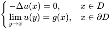
Let ${\displaystyle D}$ be a domain (an open and connected set) in $\textstyle \mathbb {R} ^{n}}$. Let ${\displaystyle \Delta }$ be the Laplace operator, let ${\displaystyle g}$ be a bounded function on the boundary${\displaystyle \partial D}$, and consider the problem:

${\displaystyle {\begin{cases}-\Delta u(x)=0,&x\in D\\\displaystyle {\lim _{y\to x}u(y)}=g(x),&x\in \partial D\end{cases}}}$

It can be shown that if a solution ${\displaystyle u}$ exists, then ${\displaystyle u(x)}$は期待値です${\displaystyle g(x)}$（ランダムな）最初の出口地点で${\displaystyle D}$標準的なブラウン運動の場合、${\displaystyle x}$定理3については、Kakutani 1944、p.710を参照のこと 。

させて${\displaystyle D}$ドメインである$\textstyle \mathbb {R} ^{n}}$そして${\displaystyle L}$半楕円微分作用素である${\textstyle C^{2}(\mathbb {R} ^{n};\mathbb {R} )}$以下の形式：

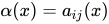
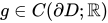
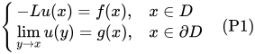
${\displaystyle L=\sum _{i=1}^{n}b_{i}(x){\frac {\partial }{\partial x_{i}}}+\sum _{i,j=1}^{n}a_{ij}(x){\frac {\partial ^{2}}{\partial x_{i}\,\partial x_{j}}}}$

ここで係数は${\displaystyle b_{i}}$そして${\displaystyle a_{ij}}$は連続関数であり、行列のすべての固有値である。${\displaystyle \alpha (x)=a_{ij}(x)}$は非負である。${\textstyle f\in C(D;\mathbb {R} )}$そして${\textstyle g\in C(\partial D;\mathbb {R} )}$ポアソン問題を考えてみましょう。

${\displaystyle {\begin{cases}-Lu(x)=f(x),&x\in D\\\displaystyle {\lim _{y\to x}u(y)}=g(x),&x\in \partial D\end{cases}}\quad {\mbox{(P1)}}}$

この問題を解決するための確率的方法の考え方は次のとおりです。まず、伊藤拡散を求めます。${\displaystyle X}$その無限小生成器${\displaystyle A}$と一致する${\displaystyle L}$コンパクトに支持された${\displaystyle C^{2}}$関数${\displaystyle f:\mathbb {R} ^{n}\rightarrow \mathbb {R} }$。 例えば、${\displaystyle X}$これは、確率微分方程式の解とみなすことができる。

${\displaystyle \mathrm {d} X_{t}=b(X_{t})\,\mathrm {d} t+\sigma (X_{t})\,\mathrm {d} B_{t}}$

どこ${\displaystyle B}$n次元ブラウン運動は、${\displaystyle b}$コンポーネントがあります${\displaystyle b_{i}}$上記のとおり、行列場${\displaystyle \sigma }$次のように選択されます。

${\displaystyle {\frac {1}{2}}\sigma (x)\sigma (x)^{\top }=a(x),\quad \forall x\in \mathbb {R} ^{n}}$

ある点については${\displaystyle x\in \mathbb {R} ^{n}}$、 させて${\displaystyle \mathbb {P} ^{x}}$法則を表す${\displaystyle X}$与えられた初期データ${\displaystyle X_{0}=x}$、そして${\displaystyle \mathbb {E} ^{x}}$に関して期待値を表す${\displaystyle \mathbb {P} ^{x}}$。 させて${\displaystyle \tau _{D}}$最初の退出時間を表す${\displaystyle X}$から${\displaystyle D}$。

この表記法では、（P1）の候補解は次のようになります。

${\displaystyle u(x)=\mathbb {E} ^{x}\left[g{\big (}X_{\tau _{D}}{\big )}\cdot \chi _{\{\tau _{D}<+\infty \}}\right]+\mathbb {E} ^{x}\left[\int _{0}^{\tau _{D}}f(X_{t})\,\mathrm {d} t\right]}$

ただし、${\displaystyle g}$は有界関数であり、以下の条件を満たす。

${\displaystyle \mathbb {E} ^{x}\left[\int _{0}^{\tau _{D}}{\big |}f(X_{t}){\big |}\,\mathrm {d} t\right]<+\infty }$

もう一つ条件が必要であることが判明した。

${\displaystyle \mathbb {P} ^{x}{\big (}\tau _{D}<\infty {\big )}=1,\quad \forall x\in D}$

すべての人にとって${\displaystyle x}$プロセス${\displaystyle X}$開始${\displaystyle x}$ほぼ確実に${\displaystyle D}$有限時間内に。この仮定の下では、上記の候補解は以下のように簡略化される。

${\displaystyle u(x)=\mathbb {E} ^{x}\left[g{\big (}X_{\tau _{D}}{\big )}\right]+\mathbb {E} ^{x}\left[\int _{0}^{\tau _{D}}f(X_{t})\,\mathrm {d} t\right]}$

そして、(P1)を解くのは、${\displaystyle {\mathcal {A}}}$は特性演算子を表す。${\displaystyle X}$（これは${\displaystyle A}$の上${\displaystyle C^{2}}$関数)、次に:

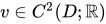
${\displaystyle {\begin{cases}-{\mathcal {A}}u(x)=f(x),&x\in D\\\displaystyle {\lim _{t\uparrow \tau _{D}}u(X_{t})}=g{\big (}X_{\tau _{D}}{\big )},&\mathbb {P} ^{x}{\mbox{-a.s.,}}\;\forall x\in D\end{cases}}\quad {\mbox{(P2)}}}$

さらに、もし${\textstyle v\in C^{2}(D;\mathbb {R} )}$（P2）を満たし、定数が存在する${\displaystyle C}$すべての${\displaystyle x\in D}$:

${\displaystyle |v(x)|\leq C\left(1+\mathbb {E} ^{x}\left[\int _{0}^{\tau _{D}}{\big |}g(X_{s}){\big |}\,\mathrm {d} s\right]\right)}$

それから${\displaystyle v=u}$。

• 角谷静雄(1944). 「二次元ブラウン運動と調和関数」 .帝国科学アカデミー紀要. 東京. 20 (10): 706–714 . doi : 10.3792/pia/1195572706 .
• 角谷静雄(1944). 「 n空間におけるブラウン運動について」 .東京都科学院紀要. 20 (9): 648–652 . doi : 10.3792/pia/1195572742 .