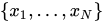
数学 において、低不一致数列 とは、すべての値に対してという性質を持つ数列のこと である。N {\displaystyle N} x 1 、 … 、 x N {\displaystyle x_{1},\ldots ,x_{N}} 不一致 が少ない。
大まかに言えば、数列の不一致度は、数列内の点が任意の集合B に収まる割合が、B の尺度 にほぼ比例する場合に低くなります。これは、平均的には(ただし、個々のサンプルではそうではありません)均等分布数列 の場合に起こります。不一致度の具体的な定義は、 B の選択(超球 、超立方体 など)や、各 B の不一致度の計算方法(通常は正規化)と結合方法(通常は最悪の値を取る)によって異なります。
低不一致数列は、一様分布乱数 の代替としてよく用いられることから、準乱数 列とも呼ばれます。「準」という修飾語は、低不一致数列の値が乱数でも擬似乱数でもないことをより明確に示すために用いられますが、このような数列は乱数の特性をいくつか共有しており、 準モンテカルロ法 などの特定のアプリケーションでは、その不一致の小ささが重要な利点となります。
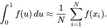
させて私 ¯ s \displaystyle {\overline {I}}^{s}} s {\displaystyle s} 単位立方体 、私 ¯ s = [ 0 、 1 ] × ⋯ × [ 0 、 1 ] {\displaystyle {\overline {I}}^{s}=[0,1]\times \cdots \times [0,1]} f {\displaystyle f} 変動範囲が限定され ているV ( f ) {\displaystyle V(f)} 私 ¯ s \displaystyle {\overline {I}}^{s}} ハーディ とクラウスの意味で。x 1 、 … 、 x N {\displaystyle x_{1},\ldots ,x_{N}} 私 s = [ 0 、 1 ) s = [ 0 、 1 ) × ⋯ × [ 0 、 1 ) {\displaystyle I^{s}=[0,1)^{s}=[0,1)\times \cdots \times [0,1)}
| 1 N ∑ 私 = 1 N f ( x 私 ) − ∫ 私 ¯ s f ( u ) d u | ≤ V ( f ) D N * ( x 1 、 … 、 x N ) 。 \displaystyle \left|{\frac {1}{N}}\sum _{i=1}^{N}f(x_{i})-\int _{{\bar {I}}^{s}}f(u)\,du\right|\leq V(f)\,D_{N}^{*}(x_{1},\ldots ,x_{N}).} フラフカの不等式は 、 次の意味で厳密である。任意の点集合に対して{ x 1 、 … 、 x N } {\displaystyle \{x_{1},\ldots ,x_{N}\}} 私 s {\displaystyle I^{s}} ε > 0 {\displaystyle \varepsilon >0} f {\displaystyle f} V ( f ) = 1 {\displaystyle V(f)=1}
| 1 N ∑ 私 = 1 N f ( x 私 ) − ∫ 私 ¯ s f ( u ) d u | > D N * ( x 1 、 … 、 x N ) − ε 。 \displaystyle \left|{\frac {1}{N}}\sum _{i=1}^{N}f(x_{i})-\int _{{\bar {I}}^{s}}f(u)\,du\right|>D_{N}^{*}(x_{1},\ldots ,x_{N})-\varepsilon .}
したがって、数値積分規則の品質は、不一致のみに依存します。D N * ( x 1 、 … 、 x N ) {\displaystyle D_{N}^{*}(x_{1},\ldots ,x_{N})}
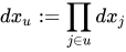
させてD = { 1 、 2 、 … 、 d } {\displaystyle D=\{1,2,\ldots ,d\}} ∅ ≠ u ⊆ D {\displaystyle \emptyset \neq u\subseteq D} d x u := ∏ j ∈ u d x j \displaystyle dx_{u}:=\prod _{j\in u}dx_{j}} ( x u 、 1 ) {\displaystyle (x_{u},1)} xから u に含まれない座標を置き換えることによって得られる点1 {\displaystyle 1}
1 N ∑ 私 = 1 N f ( x 私 ) − ∫ 私 ¯ s f ( u ) d u = ∑ ∅ ≠ u ⊆ D ( − 1 ) | u | ∫ [ 0 、 1 ] | u | ディスク ( x u 、 1 ) ∂ | u | ∂ x u f ( x u 、 1 ) d x u 、 {\displaystyle {\frac {1}{N}}\sum _{i=1}^{N}f(x_{i})-\int _{{\bar {I}}^{s}}f(u)\,du=\sum _{\emptyset \neq u\subseteq D}(-1)^{|u|}\int _{[0,1]^{|u|}}\operatorname {disc} (x_{u},1){\frac {\partial ^{|u|}}{\partial x_{u}}}f(x_{u},1)\,dx_{u},}
どこディスク ( z ) = 1 N ∑ 私 = 1 N ∏ j = 1 d 1 [ 0 、 z j ) ( x 私 、 j ) − ∏ j = 1 d z 私 {\displaystyle \operatorname {disc} (z)={\frac {1}{N}}\sum _{i=1}^{N}\prod _{j=1}^{d}1_{[0,z_{j})}(x_{i,j})-\prod _{j=1}^{d}z_{i}}
L 2バージョン 積分と和に対するコーシー・シュワルツの不等式を フラウカ・ザレンバの恒等式に適用すると、次の式が得られます。L 2 {\displaystyle L^{2}}
| 1 N ∑ 私 = 1 N f ( x 私 ) − ∫ 私 ¯ s f ( u ) d u | ≤ ‖ f ‖ d ディスク d ( { t 私 } ) 、 {\displaystyle \left|{\frac {1}{N}}\sum _{i=1}^{N}f(x_{i})-\int _{{\bar {I}}^{s}}f(u)\,du\right|\leq \|f\|_{d}\operatorname {disc} _{d}(\{t_{i}\}),}
どこ
ディスク d ( { t 私 } ) = ( ∑ ∅ ≠ u ⊆ D ∫ [ 0 、 1 ] | u | ディスク ( x u 、 1 ) 2 d x u ) 1 / 2 {\displaystyle \operatorname {disc} _{d}(\{t_{i}\})=\left(\sum _{\emptyset \neq u\subseteq D}\int _{[0,1]^{|u|}}\operatorname {disc} (x_{u},1)^{2}\,dx_{u}\right)^{1/2}}
そして
‖ f ‖ d = ( ∑ u ⊆ D ∫ [ 0 、 1 ] | u | | ∂ | u | ∂ x u f ( x u 、 1 ) | 2 d x u ) 1 / 2 。 {\displaystyle \|f\|_{d}=\left(\sum _{u\subseteq D}\int _{[0,1]^{|u|}}\left|{\frac {\partial ^{|u|}}{\partial x_{u}}}f(x_{u},1)\right|^{2}dx_{u}\right)^{1/2}.}
L 2 {\displaystyle L^{2}} L 2 {\displaystyle L^{2}}
大規模な点集合の差異の正確な値を求めるのは計算上困難である。エルデシュ ・トゥラン ・コクスマの 不等式は上限値を与える。
させてx 1 、 … 、 x N {\displaystyle x_{1},\ldots ,x_{N}} 私 s {\displaystyle I^{s}} H {\displaystyle H}
D N * ( x 1 、 … 、 x N ) ≤ ( 3 2 ) s ( 2 H + 1 + ∑ 0 < ‖ h ‖ ∞ ≤ H 1 r ( h ) | 1 N ∑ n = 1 N e 2 π 私 ⟨ h 、 x n ⟩ | ) {\displaystyle D_{N}^{*}(x_{1},\ldots ,x_{N})\leq \left({\frac {3}{2}}\right)^{s}\left({\frac {2}{H+1}}+\sum _{0<\|h\|_{\infty }\leq H}{\frac {1}{r(h)}}\left|{\frac {1}{N}}\sum _{n=1}^{N}e^{2\pi i\langle h,x_{n}\rangle }\right|\right)}
どこ
r ( h ) = ∏ 私 = 1 s 最大 { 1 、 | h 私 | } のために h = ( h 1 、 … 、 h s ) ∈ Z s 。 {\displaystyle r(h)=\prod _{i=1}^{s}\max\{1,|h_{i}|\}\quad {\text{for}}\quad h=(h_{1},\ldots ,h_{s})\in \mathbb {Z} ^{s}.}
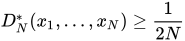
下限値 させてs = 1 {\displaystyle s=1}
D N * ( x 1 、 … 、 x N ) ≥ 1 2 N {\displaystyle D_{N}^{*}(x_{1},\ldots ,x_{N})\geq {\frac {1}{2N}}}
任意の有限点集合に対して{ x 1 、 … 、 x N } {\displaystyle \{x_{1},\dots ,x_{N}}\}
させてs = 2 {\displaystyle s=2} WM Schmidt は 、任意の有限点集合に対して、{ x 1 、 … 、 x N } {\displaystyle \{x_{1},\dots ,x_{N}}\}
D N * ( x 1 、 … 、 x N ) ≥ C ログ N N {\displaystyle D_{N}^{*}(x_{1},\ldots ,x_{N})\geq C{\frac {\log N}{N}}}
どこ
C = 最大 1 ≥ 3 1 16 1 − 2 1 ログ 1 = 0.023335 … 。 {\displaystyle C=\max _{a\geq 3}{\frac {1}{16}}{\frac {a-2}{a\log a}}=0.023335\dots .}
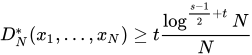
任意の寸法s > 1 {\displaystyle s>1} KFロス は、
D N * ( x 1 、 … 、 x N ) ≥ 1 2 4 s 1 ( ( s − 1 ) ログ 2 ) s − 1 2 ログ s − 1 2 N N {\displaystyle D_{N}^{*}(x_{1},\ldots ,x_{N})\geq {\frac {1}{2^{4s}}}{\frac {1}{((s-1)\log 2)^{\frac {s-1}{2}}}}{\frac {\log ^{\frac {s-1}{2}}N}{N}}}
任意の有限点集合に対して{ x 1 、 … 、 x N } {\displaystyle \{x_{1},\dots ,x_{N}}\} [ 1] M. T. Lacey to a power of a single logarithm. The best known bound for s > 2 is due D. Bilyk and M. T. Lacey and A. Vagharshakyan.[ 2] t > 0 {\displaystyle t>0} s so that D N ∗ ( x 1 , … , x N ) ≥ t log s − 1 2 + t N N {\displaystyle D_{N}^{*}(x_{1},\ldots ,x_{N})\geq t{\frac {\log ^{{\frac {s-1}{2}}+t}N}{N}}}
for any finite point set { x 1 , … , x N } {\displaystyle \{x_{1},\dots ,x_{N}}\}
Construction of low-discrepancy sequences Because any distribution of random numbers can be mapped onto a uniform distribution, and quasirandom numbers are mapped in the same way, this article only concerns generation of quasirandom numbers on a multidimensional uniform distribution.
There are constructions of sequences known such that D N ∗ ( x 1 , … , x N ) ≤ C ( ln N ) s N . {\displaystyle D_{N}^{*}(x_{1},\ldots ,x_{N})\leq C{\frac {(\ln N)^{s}}{N}}.} C {\displaystyle C} van der Corput sequence , the Halton sequences , and the Sobol’ sequences . One general limitation is that construction methods can usually only guarantee the order of convergence. Practically, low discrepancy can be only achieved if N {\displaystyle N} N {\displaystyle N} s = 20 {\displaystyle s=20} N = 1000 {\displaystyle N=1000}
Random numbers Sequences of quasirandom numbers can be generated from random numbers by imposing a negative correlation on those random numbers. One way to do this is to start with a set of random numbers r i {\displaystyle r_{i}} [ 0 , 0.5 ) {\displaystyle [0,0.5)} s i {\displaystyle s_{i}} [ 0 , 1 ) {\displaystyle [0,1)}
s i = r i {\displaystyle s_{i}=r_{i}} i {\displaystyle i} s i = 0.5 + r i {\displaystyle s_{i}=0.5+r_{i}} i {\displaystyle i}
A second way to do it with the starting random numbers is to construct a random walk with offset 0.5 as in:
s i = s i − 1 + 0.5 + r i ( mod 1 ) . {\displaystyle s_{i}=s_{i-1}+0.5+r_{i}{\pmod {1}}.\,}
That is, take the previous quasirandom number, add 0.5 and the random number, and take the result modulo 1.
For more than one dimension, Latin squares of the appropriate dimension can be used to provide offsets to ensure that the whole domain is covered evenly.
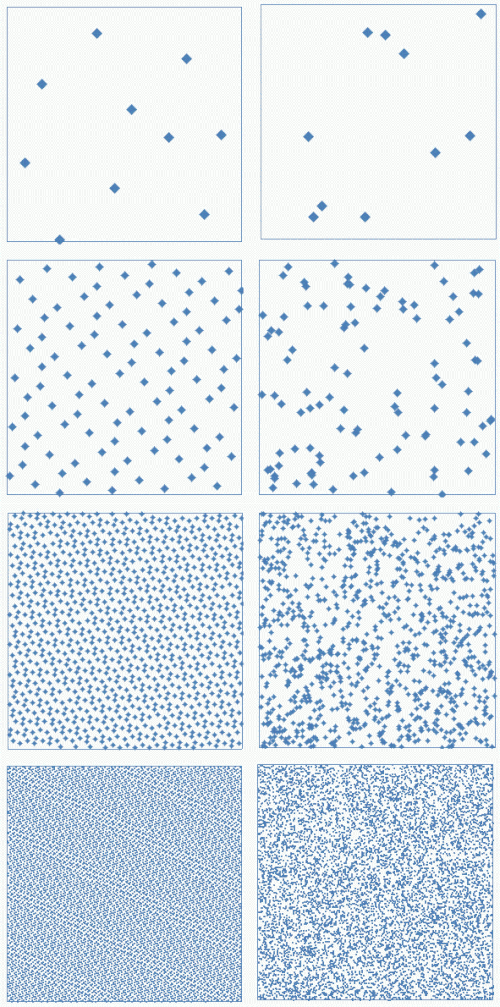
Coverage of the unit square. Left for additive quasirandom numbers with c = 0.5545497..., 0.308517... Right for random numbers. From top to bottom. 10, 100, 1000, 10000 points.
Additive recurrence For any irrational α {\displaystyle \alpha }
s n = { s 0 + n α } {\displaystyle s_{n}=\{s_{0}+n\alpha \}}
has discrepancy tending to 1 / N {\displaystyle 1/N} s n + 1 = ( s n + α ) mod 1 . {\displaystyle s_{n+1}=(s_{n}+\alpha ){\bmod {1}}\;.}
A good value of α {\displaystyle \alpha }
The discrepancy can be bounded by the approximation exponent of α {\displaystyle \alpha } μ {\displaystyle \mu } ε > 0 {\displaystyle \varepsilon >0} [ 3 ]
D N ( ( s n ) ) = O ε ( N − 1 / ( μ − 1 ) + ε ) 。 {\displaystyle D_{N}((s_{n}))=O_{\varepsilon }(N^{-1/(\mu -1)+\varepsilon }).}
チュー・ジーゲル・ロス定理 によれば、任意の無理代数的数 の近似指数は 2 であり、N − 1 + ε {\displaystyle N^{-1+\varepsilon }}
上記の漸化式は、低品質の擬似乱数生成器である線形合同法生成器 で使用される漸化式に似ています。 [ 4 ]
r 私 = ( 1 r 私 − 1 + c ) モジュール m {\displaystyle r_{i}=(ar_{i-1}+c){\bmod {m}}}
上記の低不一致加法漸化式では、a とm は1に設定されます。ただし、これは独立した乱数を生成しないため、独立性を必要とする用途には使用しないでください。
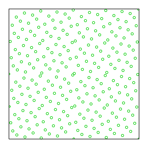
価値c {\displaystyle c} 黄金比 の小数部分 です: [ 5 ]
c = 5 − 1 2 = φ − 1 ≈ 0.618034。 {\displaystyle c={\frac {{\sqrt {5}}-1}{2}}=\varphi -1\approx 0.618034.}
ほぼ同等の精度を持つ別の値は、銀比率 の小数部分、つまり2の平方根の小数部分です。
c = 2 − 1 ≈ 0.414214。 {\displaystyle c={\sqrt {2}}-1\approx 0.414214.\,}
複数の次元の場合、各次元ごとに個別の準乱数が必要になります。よく使われる便利な値のセットは、2以上の素数の平方根をすべて1で割ったものです。
c = 2 、 3 、 5 、 7 、 11 、 … {\displaystyle c={\sqrt {2}},{\sqrt {3}},{\sqrt {5}},{\sqrt {7}},{\sqrt {11}},\ldots \,}
しかし、一般化された黄金比に基づく一連の値は、より均等に分布した点を生成することが示されている。[ 6 ]
擬似乱数生成器のリストには、 独立した擬似乱数を生成する方法が一覧表示されています。 注 :次元が少ない場合、再帰的反復法は良質な均一集合を生成しますが、次元が大きい場合はs {\displaystyle s} s > 8 {\displaystyle s>8}
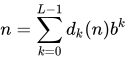
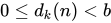
ファン・デル・コルプト系列 させて
n = ∑ k = 0 L − 1 d k ( n ) b k {\displaystyle n=\sum _{k=0}^{L-1}d_{k}(n)b^{k}}
になるb {\displaystyle b} n ≥ 1 {\displaystyle n\geq 1} 0 ≤ d k ( n ) < b {\displaystyle 0\leq d_{k}(n)<b}
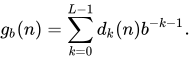
g b ( n ) = ∑ k = 0 L − 1 d k ( n ) b − k − 1 。 {\displaystyle g_{b}(n)=\sum _{k=0}^{L-1}d_{k}(n)b^{-k-1}.}
そして定数があるC {\displaystyle C} b {\displaystyle b} ( g b ( n ) ) n ≥ 1 {\displaystyle (g_{b}(n))_{n\geq 1}}
D N * ( g b ( 1 ) 、 … 、 g b ( N ) ) ≤ C ログ N N 、 {\displaystyle D_{N}^{*}(g_{b}(1),\dots ,g_{b}(N))\leq C{\frac {\log N}{N}},}
どこD N * {\displaystyle D_{N}^{*}} 星の不一致
ハルトンシーケンス (2,3)ハルトン数列の最初の256点 ハルトン数列は、ファン・デル・コルプト数列を高次元に自然に一般化したものである。sを 任意の次元とし、b 1 , ..., b s を 互いに素 な整数とする。
x ( n ) = ( g b 1 ( n ) 、 … 、 g b s ( n ) ) 。 {\displaystyle x(n)=(g_{b_{1}}(n),\dots ,g_{b_{s}}(n)).}
すると、b 1 、 ...、b s C が存在し、シーケンス { x ( n )} n ≥1 はs 次元シーケンスで、
D N * ( x ( 1 ) 、 … 、 x ( N ) ) ≤ C ′ ( ログ N ) s N 。 {\displaystyle D_{N}^{*}(x(1),\dots ,x(N))\leq C'{\frac {(\log N)^{s}}{N}}.}
ハマーズリーがセット 2D ハマーリーセット サイズ256 させてb 1 、 … 、 b s − 1 {\displaystyle b_{1},\ldots ,b_{s-1}} 互いに素な 1より大きい正の整数とする。s {\displaystyle s} N {\displaystyle N} s {\displaystyle s} ハマーズリー セットのサイズN {\displaystyle N} [ 7 ]
x ( n ) = ( g b 1 ( n ) 、 … 、 g b s − 1 ( n ) 、 n N ) {\displaystyle x(n)=\left(g_{b_{1}}(n),\dots ,g_{b_{s-1}}(n),{\frac {n}{N}}\right)}
のためにn = 1 、 … 、 N {\displaystyle n=1,\ldots ,N}
D N * ( x ( 1 ) 、 … 、 x ( N ) ) ≤ C ( ログ N ) s − 1 N {\displaystyle D_{N}^{*}(x(1),\dots ,x(N))\leq C{\frac {(\log N)^{s-1}}{N}}}
どこC {\displaystyle C} b 1 、 … 、 b s − 1 {\displaystyle b_{1},\ldots ,b_{s-1}}
注 :式から、ハマーズリー集合は実際にはハルトン数列であることがわかりますが、線形掃引を追加することで次元が1つ増えます。これは、次の場合にのみ可能です。 N {\displaystyle N} s = 2 {\displaystyle s=2}
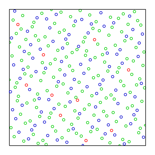
ポアソンディスクサンプリング ポアソンディスクサンプリングは 、ビデオゲームでよく用いられ、ランダムに見えるようにオブジェクトを素早く配置しながら、任意の2点が少なくとも指定された最小距離以上離れていることを保証する。[ 8 ] 周波数分析 に基づいており、いわゆる「ブルーノイズ」パターンの一種である。
グラフィカルな例 下に示した点は、Sobol' 型のシーケンスの最初の 100、1000、および 10000 要素です。比較のために、擬似乱数点のシーケンスの 10000 要素も示しています。低不一致シーケンスは、TOMS アルゴリズム 659によって生成されました。 [ 9 ] Fortran でのアルゴリズムの実装はNetlib から入手できます。
注記 ↑ ベック、ヨーゼフ (1989)。「分布の不規則性における 2 次元のファン・アーデンヌ・エーレンフェストの定理」。Compositio Mathematica 。72 ( 3) : 269–339。MR 1032337 。 S2CID 125940424。Zbl 0691.10041。 ↑ Bilyk, Dmitriy; Lacey, Michael T.; Vagharshakyan, Armen (2008). "On the Small Ball Inequality in all dimensions" . Journal of Functional Analysis . 254 (9): 2470–2502 . arXiv : 0705.4619 . doi : 10.1016/j.jfa.2007.09.010 . S2CID 14234006 . ↑ カイパースと ニーダーライター、2005 年 、p. 123 ↑ ドナルド・E・クヌース 「第3章 – 乱数」 『コンピュータプログラミングの技法 』第 2巻。 ↑ スカルプケ、マルテ(2018年6月16日) 「フィボナッチハッシュ:世界が忘れた最適化」 。 黄金比の特性の一つは、事前に何ステップ進むか分からない場合でも、任意の範囲をほぼ均等に分割できることである。 ↑ ロバーツ、マーティン (2018)。 「準ランダムシーケンスの不合理な有効性」 。 2025年3月1日に オリジナル からアーカイブされました。 ↑ Hammersley, JM; Handscomb, DC (1964). Monte Carlo Methods . doi : 10.1007/978-94-009-5819-7 . ISBN 978-94-009-5821-0 。↑ ハーマン・タレンケン。 ハーマン、タレンケン(2008 年 3 月)。 「ポアソンディスクサンプリング」 。 開発雑誌 。 No. 21。21 ~ 25ページ 。 ↑ Bratley, Paul; Fox, Bennett L. (1988). "アルゴリズム 659" . ACM Transactions on Mathematical Software . 14 : 88– 100. doi : 10.1145/42288.214372 . S2CID 17325779 .
参考文献 ディック、ヨーゼフ、ピリヒシャマー、フリードリヒ(2010)。デジタルネットとシーケンス:不一致理論と準モンテカルロ積分 。ケンブリッジ大学出版局。ISBN 978-0-521-19159-3 。 カイパーズ、L. Niederreiter, H. (2005)、配列の均一分布 、Dover Publications 、ISBN 0-486-45019-8 ハラルド・ニーダーライター (1992)。乱数生成と準モンテカルロ法 。応用数理学会。ISBN 0-89871-295-5 。Drmota, Michael; Tichy, Robert F. (1997).数列、不一致、および応用 . Lecture Notes in Math. Vol. 1651. Springer. ISBN 3-540-62606-9 。 Press, William H.; Flannery, Brian P.; Teukolsky, Saul A.; Vetterling, William T. (1992). Numerical Recipes in C ed.). Cambridge University Press. 低不一致数列に関するより専門的な説明については、セクション 7.7 を参照してください。ISBN 0-521-43108-5 。
外部リンク ACMアルゴリズム集(アルゴリズム647、659、738を参照。) GNU科学ライブラリ からの準ランダムシーケンスFinancialMathematics.Com の制約条件付き準ランダムサンプリング C++によるソボル数列生成器 SciPy QMC APIリファレンス:scipy.stats.qmc 















![{\displaystyle {\overline {I}}^{s}=[0,1]\times \cdots \times [0,1]}](https://wikimedia.org/api/rest_v1/media/math/render/svg/b7b6b45832d30cbe2b66656b80245cb209cb4262)











![{\displaystyle {\frac {1}{N}}\sum _{i=1}^{N}f(x_{i})-\int _{{\bar {I}}^{s}}f(u)\,du=\sum _{\emptyset \neq u\subseteq D}(-1)^{|u|}\int _{[0,1]^{|u|}}\operatorname {disc} (x_{u},1){\frac {\partial ^{|u|}}{\partial x_{u}}}f(x_{u},1)\,dx_{u},}](https://wikimedia.org/api/rest_v1/media/math/render/svg/646d05c4c12cae58e128651816856d90c9a25e51)


![{\displaystyle \operatorname {disc} _{d}(\{t_{i}\})=\left(\sum _{\emptyset \neq u\subseteq D}\int _{[0,1]^{|u|}}\operatorname {disc} (x_{u},1)^{2}\,dx_{u}\right)^{1/2}}](https://wikimedia.org/api/rest_v1/media/math/render/svg/609a886b91fa44773d2ddd89c752bc1a037309a6)
![{\displaystyle \|f\|_{d}=\left(\sum _{u\subseteq D}\int _{[0,1]^{|u|}}\left|{\frac {\partial ^{|u|}}{\partial x_{u}}}f(x_{u},1)\right|^{2}dx_{u}\right)^{1/2}.}](https://wikimedia.org/api/rest_v1/media/math/render/svg/dee8232a0985af6392e00e77e9bdfa8c4f98fe77)