一般化フーリエ級数

一般化フーリエ級数は、二乗積分可能関数を二乗積分可能直交基底関数の和に展開したものである。標準フーリエ級数は三角関数の正規直交基底を使用し、級数展開は周期関数に適用される。対照的に、一般化フーリエ級数は任意の直交基底関数のセットを使用し、任意の二乗積分可能関数に適用できる。^{[1] [2]}

閉区間上で定義され、重み付き内積の下で直交する2乗積分可能な複素数値関数の集合を考える。 ${\displaystyle \Phi =\{\phi _{n}:[a,b]\to \mathbb {C} \}_{n=0}^{\infty }}$${\displaystyle [a,b]}$

${\displaystyle \langle f,g\rangle _{w}=\int _{a}^{b}f(x){\overline {g(x)}}w(x)dx,}$

ここで、 は重み関数であり、は の複素共役です。関数の一般化フーリエ級数は、次のようになります。 ここで、係数は次のように与えられます。 ${\displaystyle w(x)}$${\displaystyle {\overline {g}}}$${\displaystyle g}$${\displaystyle f}$$${\displaystyle f(x)=\sum _{n=0}^{\infty }c_{n}\phi _{n}(x),}$$$${\displaystyle c_{n}={\langle f,\phi _{n}\rangle _{w} \over \|\phi _{n}\|_{w}^{2}}.}$$

与えられた区間上で定義された平方可積分関数の空間が与えられれば、区間上の境界値問題のクラス、いわゆる正則ストゥルム・リウヴィル問題を考えることによって直交基底を見つけることができます。これらは次のように定義されます。 ここで、および はおよび上で連続な実数であり、および は自己随伴境界条件であり、 は上の正の連続関数です。 ${\displaystyle L^{2}(a,b)}$${\displaystyle [a,b]}$$${\displaystyle (rf')'+pf+\lambda wf=0}$$ $${\displaystyle B_{1}(f)=B_{2}(f)=0}$$${\displaystyle r,r'}$${\displaystyle p}$${\displaystyle [a,b]}$${\displaystyle r>0}$${\displaystyle [a,b]}$${\displaystyle B_{1}}$${\displaystyle B_{2}}$${\displaystyle w}$${\displaystyle [a,b]}$

上記で定義した正則ストゥルム・リウヴィル問題を考えると、問題の異なる固有値解に対応する固有関数の集合は、重み付き内積に関して の直交基底を形成します。^[3]また、このストゥルム・リウヴィル問題の境界条件を満たす関数については、級数が に一様に収束することもわかります。^[4]${\displaystyle \{\phi _{n}\}_{1}^{\infty }}$${\displaystyle L^{2}(a,b)}$${\displaystyle \langle \cdot ,\cdot \rangle _{w}}$${\displaystyle f\in L^{2}(a,b)}$${\displaystyle \sum _{n=1}^{\infty }\langle f,\phi _{n}\rangle \phi _{n}}$ ${\displaystyle f}$

数直線全体上で定義された関数は、任意の実数 に対して等式が成り立つような数が存在する場合、周期を持つ周期関数と呼ばれます。 ${\displaystyle f(x)}$${\displaystyle T}$${\displaystyle T>0}$${\displaystyle x}$${\displaystyle f(x+T)=f(x)}$

関数が周期 で周期的である場合、周期、、などでも周期的です。通常、関数の周期はそのような最小の数として理解されます。ただし、一部の関数では、 の任意の小さな値が存在します。 ${\displaystyle T}$${\displaystyle 2T}$${\displaystyle 3T}$${\displaystyle T}$${\displaystyle T}$

関数の列は三角関数システムとして知られています。三角関数システムの関数の任意の線形結合（無限結合（つまり、収束する無限級数）を含む）は、周期が 2π の周期関数です。 ${\displaystyle 1,\cos(x),\sin(x),\cos(2x),\sin(2x),...,\cos(nx),\sin(nx),...}$

長さ 2π の任意の線分（線分 [−π,π] や [0,2π] など）では、三角関数系は直交系です。つまり、三角関数系の任意の 2 つの関数について、長さ 2π の線分上の積分の積分はゼロになります。この積分は、長さ 2π の特定の線分上で積分可能な関数の空間における スカラー積として扱うことができます。

関数を線分 [−π, π] 上で定義します。適切な滑らかさと微分可能性の条件が与えられれば、この線分上では三角関数系の関数の線形結合として表すことができます。これは関数の三角フーリエ級数への 展開とも呼ばれます。${\displaystyle f(x)}$${\displaystyle f(x)}$${\displaystyle f(x)}$

ルジャンドル多項式は、 シュトゥルム・リウヴィルの固有値問題 の解である。${\displaystyle P_{n}(x)}$

${\displaystyle \left((1-x^{2})P_{n}'(x)\right)'+n(n+1)P_{n}(x)=0.}$

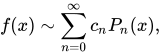
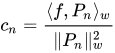
シュトゥルム・リウヴィル理論の結果として、これらの多項式は単位重みの内積に関して直交する固有関数である。これはルジャンドル多項式を含む一般化されたフーリエ級数（この場合はフーリエ・ルジャンドル級数として知られる）として記述することができ、

${\displaystyle f(x)\sim \sum _{n=0}^{\infty }c_{n}P_{n}(x),}$

${\displaystyle c_{n}={\langle f,P_{n}\rangle _{w} \over \|P_{n}\|_{w}^{2}}}$

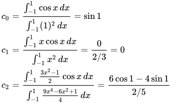
例えば、フーリエ・ルジャンドル級数は に対して計算できる。すると、 ${\displaystyle f(x)=\cos x}$${\displaystyle [-1,1]}$

${\displaystyle {\begin{aligned}c_{0}&={\int _{-1}^{1}\cos {x}\,dx \over \int _{-1}^{1}(1)^{2}\,dx}=\sin {1}\\c_{1}&={\int _{-1}^{1}x\cos {x}\,dx \over \int _{-1}^{1}x^{2}\,dx}={0 \over 2/3}=0\\c_{2}&={\int _{-1}^{1}{3x^{2}-1 \over 2}\cos {x}\,dx \over \int _{-1}^{1}{9x^{4}-6x^{2}+1 \over 4}\,dx}={6\cos {1}-4\sin {1} \over 2/5}\end{aligned}}}$

これらの項のみを含む短縮された系列は

${\displaystyle {\begin{aligned}c_{2}P_{2}(x)+c_{1}P_{1}(x)+c_{0}P_{0}(x)&={5 \over 2}(6\cos {1}-4\sin {1})\left({3x^{2}-1 \over 2}\right)+\sin 1\\&=\left({45 \over 2}\cos {1}-15\sin {1}\right)x^{2}+6\sin {1}-{15 \over 2}\cos {1}\end{aligned}}}$

これは、約 0.003 異なります。計算アプリケーションでは、級数展開の基底関数がすべて多項式であるため、積分と係数の計算が容易になる可能性があるため、フーリエ級数ではなくこのようなフーリエ–ルジャンドル級数を使用する方が有利な場合があります。 ${\displaystyle \cos x}$

級数の係数に関するいくつかの定理は次のとおりです。 ${\displaystyle c_{n}}$

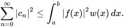
ベッセルの不等式は、ヒルベルト空間の要素の正規直交列に対する係数に関する記述である。この不等式は1828年にFWベッセルによって導かれた: ^[5]${\displaystyle x}$

${\displaystyle \sum _{n=0}^{\infty }|c_{n}|^{2}\leq \int _{a}^{b}|f(x)|^{2}w(x)\,dx.}$

パーセバルの定理は、通常、フーリエ変換がユニタリであるという結果を指します。大まかに言えば、関数の2乗の和（または積分）は、その変換の2乗の和（または積分）に等しいということです。^[6]

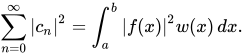
Φ が完全基底の場合、次のようになります。

${\displaystyle \sum _{n=0}^{\infty }|c_{n}|^{2}=\int _{a}^{b}|f(x)|^{2}w(x)\,dx.}$

• バナッハ空間
• 固有関数
• 分数フーリエ変換
• 機能スペース
• ヒルベルト空間
• 最小二乗スペクトル解析
• 直交関数
• 直交性
• 位相ベクトル空間
• ベクトル空間

• MathWorldの一般化フーリエ級数
• Herman, Russell (2016). フーリエ解析と複素解析入門および信号のスペクトル解析への応用(PDF) p. 73-112.
• Folland, Gerald B. (1992). フーリエ解析とその応用(PDF) . カリフォルニア州パシフィックグローブ: Wadsworth & Brooks/Cole Advanced Books & Software. p. 62-97.