幾何学 において 、 付値とは 、集合 の部分集合の集合から アーベル 半群 への有限加法関数です。たとえば、 ルベーグ測度はの 凸体 の有限和上の付値です 。 の凸体の有限和上の付値のその他の例としては、 表面積 、 平均 幅、 オイラー特性 など があります 。
バツ
{\displaystyle X}
R
ん
。
{\displaystyle \mathbb {R} ^{n}.}
R
ん
{\displaystyle \mathbb {R} ^{n}}
幾何学では、 連続性 (または 滑らかさ )条件が付値に課されることが多いが、理論の完全に離散的な側面もある。実際、付値の概念は 多面体 の分割理論、特に ヒルベルトの第3問題 に起源を持ち、抽象代数のツールに依存する豊かな理論に成長した。
意味 を集合とし 、 をの 部分集合の集合とする。 アーベル半群に値を持つ関数は、 と が の要素であるとき 、 を満たす
とき、 付値と 呼ばれる。
ならば 、常に と仮定する。
バツ
{\displaystyle X}
S
{\displaystyle {\mathcal {S}}}
バツ 。
{\displaystyle X.}
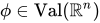
ϕ
{\displaystyle \phi}
S
{\displaystyle {\mathcal {S}}}
R
{\displaystyle R}
ϕ ( あ ∪ B ) + ϕ ( あ ∩ B ) = ϕ ( あ ) + ϕ ( B )
{\displaystyle \phi (A\cup B)+\phi (A\cap B)=\phi (A)+\phi (B)}
あ 、
{\displaystyle A,}
B 、
{\displaystyle B,}
あ ∪ B 、
{\displaystyle A\cup B,}
あ ∩ B
{\displaystyle A\cap B}
S
。
{\displaystyle {\mathcal {S}}.}
∅ ∈
S
、
{\displaystyle \emptyset \in {\mathcal {S}},}
ϕ ( ∅ ) = 0.
{\displaystyle \phi (\emptyset )=0.}
例 よくある例として は
S
{\displaystyle {\mathcal {S}}}
凸状 の 物体
R
ん
{\displaystyle \mathbb {R} ^{n}}
コンパクトな 凸 多面体
R
ん
{\displaystyle \mathbb {R} ^{n}}
凸円錐 滑らかな多様体内の滑らかなコンパクト多面体
バツ
{\displaystyle X}
を の凸体の集合と
する 。すると のいくつかの値 は
け
(
R
ん
)
{\displaystyle {\mathcal {K}}(\mathbb {R} ^{n})}
R
ん
。
{\displaystyle \mathbb {R} ^{n}.}
け
(
R
ん
)
{\displaystyle {\mathcal {K}}(\mathbb {R} ^{n})}
オイラー 特性
χ : け (
R
ん
) →
ず
{\displaystyle \chi :K(\mathbb {R} ^{n})\to \mathbb {Z} }
ルベーグ測度 は
け
(
R
ん
)
{\displaystyle {\mathcal {K}}(\mathbb {R} ^{n})}
固有体積 (より一般的には 混合体積 ) サポート 関数 が どこにあるかの 地図
あ ↦
h
あ
、
{\displaystyle A\mapsto h_{A},}
h
あ
{\displaystyle h_{A}}
あ
{\displaystyle A}
その他の評価としては
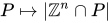
格子点列挙子 、ここでは 格子多面体
ポ ↦
|
ず
ん
∩ ポ
|
{\displaystyle P\mapsto |\mathbb {Z} ^{n}\cap P|}
ポ
{\displaystyle P}
有限集合族上の 濃度
凸体の評価 ここからは、 、 内の凸体の集合 、 上の付値とします 。
五 =
R
ん
{\displaystyle V=\mathbb {R} ^{n}}
け
( 五 )
{\displaystyle {\mathcal {K}}(V)}
五
{\displaystyle V}
ϕ
{\displaystyle \phi}
け
( 五 )
{\displaystyle {\mathcal {K}}(V)}
すべての および に対して が成り立つとき 、は 変換不変で ある と いいます 。
ϕ
{\displaystyle \phi}
け ∈
け
( 五 )
{\displaystyle K\in {\mathcal {K}}(V)}
x ∈ 五
{\displaystyle x\in V}
ϕ ( け + x ) = ϕ ( け )
{\displaystyle \phi (K+x)=\phi (K)}
とします 。 ハウスドルフ距離は 、ユークリッド内積の下で の 近傍 で
ある として定義されます
。この測定基準を備えた は、 局所的にコンパクトな空間 です 。
( け 、 ら ) ∈
け
( 五
)
2
{\displaystyle (K,L)\in {\mathcal {K}}(V)^{2}}
d
H
( け 、 ら )
{\displaystyle d_{H}(K,L)}
d
H
( け 、 ら ) = 無限大 { ε > 0 : け ⊂
ら
ε
そして
ら ⊂
け
ε
} 、
{\displaystyle d_{H}(K,L)=\inf\{\varepsilon >0:K\subset L_{\varepsilon }{\text{ および }}L\subset K_{\varepsilon }\},}
け
ε
{\displaystyle K_{\varepsilon }}
ε
{\displaystyle \epsilon }
け
{\displaystyle K}
け
( 五 )
{\displaystyle {\mathcal {K}}(V)}
からへ の連続的かつ並進不変な値空間は 次のように表される。
け
( 五 )
{\displaystyle {\mathcal {K}}(V)}
C
{\displaystyle \mathbb {C} }
ヴァル ( 五 ) 。
{\displaystyle \operatorname {Val} (V).}
上の位相は 、 のコンパクト部分集合上の一様収束の位相です。
は 、内部が空でない有界部分 集合であるノルムを備え
、 は バナッハ空間 です 。
ヴァル ( 五 )
{\displaystyle \operatorname {Val} (V)}
け
( 五 ) 。
{\displaystyle {\mathcal {K}}(V).}
‖ ϕ ‖ = 最大 {
|
ϕ ( け )
|
: け ⊂ B } 、
{\displaystyle \|\phi \|=\max\{|\phi (K)|:K\subset B\},}
B ⊂ 五
{\displaystyle B\subset V}
ヴァル ( 五 )
{\displaystyle \operatorname {Val} (V)}
均質な評価 変換不変連続値は、
すべてのに対して であるとき
、 同次 であるという。同次値 の 部分 集合は
、 マクマレンの 分解定理 [1] のベクトル部分空間である。
ϕ ∈ ヴァル ( 五 )
{\displaystyle \phi \in \operatorname {Val} (V)}
私
{\displaystyle i}
ϕ ( λ け ) =
λ
私
ϕ ( け )
{\displaystyle \phi (\lambda K)=\lambda ^{i}\phi (K)}
λ > 0
{\displaystyle \lambda >0}
け ∈
け
( 五 ) 。
{\displaystyle K\in {\mathcal {K}}(V).}
ヴァル
私
( 五 )
{\displaystyle \operatorname {Val} _{i}(V)}
私
{\displaystyle i}
ヴァル ( 五 ) 。
{\displaystyle \operatorname {Val} (V).}
ヴァル ( 五 ) =
⨁
私 = 0
ん
ヴァル
私
( 五 ) 、 ん = 薄暗い 五 。
{\displaystyle \operatorname {Val} (V)=\bigoplus _{i=0}^{n}\operatorname {Val} _{i}(V),\qquad n=\dim V.}
特に、同次評価の次数は常に との間の整数である。
0
{\displaystyle 0}
ん = 薄暗い 五 。
{\displaystyle n=\operatorname {dim} V.}
評価は、同次性の度合いだけでなく、原点を通る反射に関する偶奇性、つまり、すべての凸体に対して である場合に限り となることによっても等級付けされます
。 および の 元
は 、それぞれ 偶数 および 奇数 であると言われています 。
ヴァル
私
=
ヴァル
私
+
⊕
ヴァル
私
−
、
{\displaystyle \operatorname {Val} _{i}=\operatorname {Val} _{i}^{+}\oplus \operatorname {Val} _{i}^{-},}
ϕ ∈
ヴァル
私
ϵ
{\displaystyle \phi \in \operatorname {Val} _{i}^{\epsilon }}
ϵ ∈ { + 、 − }
{\displaystyle \epsilon \in \{+,-\}}
ϕ ( − け ) = ϵ ϕ ( け )
{\displaystyle \phi (-K)=\epsilon \phi (K)}
け 。
{\displaystyle K.}
ヴァル
私
+
{\displaystyle \operatorname {Val} _{i}^{+}}
ヴァル
私
−
{\displaystyle \operatorname {Val} _{i}^{-}}
これは、次元であり 、オイラー特性によって張られる 単純な事実であり 、つまり、定数値から構成される。
Val
0
(
V
)
{\displaystyle \operatorname {Val} _{0}(V)}
1
{\displaystyle 1}
χ
,
{\displaystyle \chi ,}
K
(
V
)
.
{\displaystyle {\mathcal {K}}(V).}
1957年に ハドヴィガー [2] は、 (ここで )が ルベーグ測度の -次元空間と一致する ことを証明した。
Val
n
(
V
)
{\displaystyle \operatorname {Val} _{n}(V)}
n
=
dim
V
{\displaystyle n=\dim V}
1
{\displaystyle 1}
V
.
{\displaystyle V.}
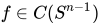
が単純な評価とは、 を持つすべての凸体に対してであるときです。Schneider [3] は 1996 年に 上のすべての単純な評価について説明しました。これらは によって与えられます。ここで は単位 球面 上 の 任意 の 奇 関数 で あり 、 は の表面積測度です。 特に、任意の単純な評価は、 - および -同次評価の和です。これは、 - 同次評価がすべての - 次元部分空間への制限によって一意に決定されること を意味します 。
ϕ
∈
Val
(
R
n
)
{\displaystyle \phi \in \operatorname {Val} (\mathbb {R} ^{n})}
ϕ
(
K
)
=
0
{\displaystyle \phi (K)=0}
dim
K
<
n
.
{\displaystyle \dim K<n.}
R
n
{\displaystyle \mathbb {R} ^{n}}
ϕ
(
K
)
=
c
vol
(
K
)
+
∫
S
n
−
1
f
(
θ
)
d
σ
K
(
θ
)
,
{\displaystyle \phi (K)=c\operatorname {vol} (K)+\int _{S^{n-1}}f(\theta )d\sigma _{K}(\theta ),}
c
∈
C
,
{\displaystyle c\in \mathbb {C} ,}
f
∈
C
(
S
n
−
1
)
{\displaystyle f\in C(S^{n-1})}
S
n
−
1
⊂
R
n
,
{\displaystyle S^{n-1}\subset \mathbb {R} ^{n},}
σ
K
{\displaystyle \sigma _{K}}
K
.
{\displaystyle K.}
n
{\displaystyle n}
(
n
−
1
)
{\displaystyle (n-1)}
i
{\displaystyle i}
(
i
+
1
)
{\displaystyle (i+1)}
埋め込み定理 クレイン埋め込みは、 偶数同次値の空間を、の -次元 線形部分 空間のグラスマン多様体上 の標準複素線束の連続セクションの空間に線型に注入するものである 。その構築は、ハドヴィガーの -同次値 の キャラクタリゼーション [2] に基づいている。および の場合、制限は 要素であり 、ハドヴィガーの定理により、それはルベーグ測度である。したがって、
上の
線束の連続セクションを定義し 、 上 のファイバーは 上の -次元密度 空間 ( ルベーグ測度) に等しい。
Val
i
+
(
V
)
,
{\displaystyle \operatorname {Val} _{i}^{+}(V),}
i
{\displaystyle i}
Gr
i
(
V
)
{\displaystyle \operatorname {Gr} _{i}(V)}
i
{\displaystyle i}
V
.
{\displaystyle V.}
n
{\displaystyle n}
ϕ
∈
Val
i
(
V
)
{\displaystyle \phi \in \operatorname {Val} _{i}(V)}
E
∈
Gr
i
(
V
)
,
{\displaystyle E\in \operatorname {Gr} _{i}(V),}
ϕ
|
E
{\displaystyle \phi |_{E}}
Val
i
(
E
)
,
{\displaystyle \operatorname {Val} _{i}(E),}
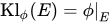
Kl
ϕ
(
E
)
=
ϕ
|
E
{\displaystyle \operatorname {Kl} _{\phi }(E)=\phi |_{E}}
D
e
n
s
{\displaystyle Dens}
Gr
i
(
V
)
{\displaystyle \operatorname {Gr} _{i}(V)}
E
{\displaystyle E}
1
{\displaystyle 1}
Dens
(
E
)
{\displaystyle \operatorname {Dens} (E)}
E
.
{\displaystyle E.}
定理 (クレイン [4] )。線型写像 は単射である。
Kl
:
Val
i
+
(
V
)
→
C
(
Gr
i
(
V
)
,
Dens
)
{\displaystyle \operatorname {Kl} :\operatorname {Val} _{i}^{+}(V)\to C(\operatorname {Gr} _{i}(V),\operatorname {Dens} )}
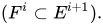
奇数値に対しては、シュナイダー埋め込みと呼ばれる別の注入が存在する。これは、シュナイダーの単純値の記述に基づいている。 [3] これは、奇同次値の空間 を、共配向ペアの部分旗多様体上の直線束の連続セクションの空間の特定の商に 線形注入するものである。その定義はクライン埋め込みを彷彿とさせるが、より複雑である。詳細は [5] を参照のこと。
Val
i
−
(
V
)
,
{\displaystyle \operatorname {Val} _{i}^{-}(V),}
i
{\displaystyle i}
(
F
i
⊂
E
i
+
1
)
.
{\displaystyle (F^{i}\subset E^{i+1}).}
グッディ・ヴェイユ埋め込みは、次元球面 の - 倍積上の超 関数空間への の線形注入である 。これは、 任意のが許容する自然な分極の シュワルツ核 、すなわち、滑らかな凸体のサポート関数の差の幾何学的意味を持つ後者の関数空間 の - 倍積上の関数としてに他ならない。詳細については、 [5] を参照。
Val
i
{\displaystyle \operatorname {Val} _{i}}
i
{\displaystyle i}
(
n
−
1
)
{\displaystyle (n-1)}
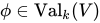
ϕ
∈
Val
k
(
V
)
{\displaystyle \phi \in \operatorname {Val} _{k}(V)}
k
{\displaystyle k}
C
2
(
S
n
−
1
)
,
{\displaystyle C^{2}(S^{n-1}),}
既約定理 ハドヴィガー、シュナイダー、マクマレンの古典的な定理は、次数 と次数に関して同次な付値についてかなり明確な説明を与えている。 しかし、 21世紀に入るまで次数についてはほとんど知られていなかった。マクマレンの予想とは、付値が
の稠密な部分空間に広がるという主張である。マクマレンの予想は、 アレスカー によってより強力な形で確認され 、既約性定理として知られるようになった。
1
,
{\displaystyle 1,}
n
−
1
,
{\displaystyle n-1,}
n
=
dim
V
.
{\displaystyle n=\operatorname {dim} V.}
1
<
i
<
n
−
1
{\displaystyle 1<i<n-1}
ϕ
A
(
K
)
=
vol
n
(
K
+
A
)
,
A
∈
K
(
V
)
,
{\displaystyle \phi _{A}(K)=\operatorname {vol} _{n}(K+A),\qquad A\in {\mathcal {K}}(V),}
Val
(
V
)
.
{\displaystyle \operatorname {Val} (V).}
定理 (アレスカー [6] )。任意の 空間 および上 の自然な作用は 既約である。
0
≤
i
≤
n
,
{\displaystyle 0\leq i\leq n,}
G
L
(
V
)
{\displaystyle GL(V)}
Val
i
+
(
V
)
{\displaystyle \operatorname {Val} _{i}^{+}(V)}
Val
i
−
(
V
)
{\displaystyle \operatorname {Val} _{i}^{-}(V)}
ここで、一般線型群 のへ の作用は次 のように与えられます。
既約性定理の証明は、前のセクションの埋め込み定理と Beilinson-Bernstein の局在 に基づいています。
G
L
(
V
)
{\displaystyle GL(V)}
Val
(
V
)
{\displaystyle \operatorname {Val} (V)}
(
g
⋅
ϕ
)
(
K
)
=
ϕ
(
g
−
1
K
)
.
{\displaystyle (g\cdot \phi )(K)=\phi (g^{-1}K).}
スムーズな評価 からへ の 写像が滑らかな場合、 付値は 滑らか と呼ばれます 。言い換えると、 が滑らかであるためには、 が の自然な表現の滑らかなベクトルである場合 に 限り ます。 滑らかな付値の空間はで稠密です 。それは自然なフレシェ空間位相を備えており、これは から誘導されるものよりも細かいものです。
ϕ
∈
Val
(
V
)
{\displaystyle \phi \in \operatorname {Val} (V)}
g
↦
g
⋅
ϕ
{\displaystyle g\mapsto g\cdot \phi }
G
L
(
V
)
{\displaystyle GL(V)}
Val
(
V
)
{\displaystyle \operatorname {Val} (V)}
ϕ
{\displaystyle \phi }
ϕ
{\displaystyle \phi }
G
L
(
V
)
{\displaystyle GL(V)}
Val
(
V
)
.
{\displaystyle \operatorname {Val} (V).}
Val
∞
(
V
)
{\displaystyle \operatorname {Val} ^{\infty }(V)}
Val
(
V
)
{\displaystyle \operatorname {Val} (V)}
Val
(
V
)
.
{\displaystyle \operatorname {Val} (V).}
上の すべての(複素数値)滑らかな関数(
ここで、は 直交射影を表し、 はハール測度)に対して、次数の滑らかな偶数値を定義します。カッセルマン・ワラッハの定理と組み合わせた既約定理から、任意の滑らかな偶数値はこのように表すことができます。このような表現は、 クロフトンの公式 と呼ばれることもあります 。
f
{\displaystyle f}
Gr
i
(
R
n
)
,
{\displaystyle \operatorname {Gr} _{i}(\mathbb {R} ^{n}),}
ϕ
(
K
)
=
∫
Gr
i
(
R
n
)
vol
i
(
P
E
K
)
f
(
E
)
d
E
,
{\displaystyle \phi (K)=\int _{\operatorname {Gr} _{i}(\mathbb {R} ^{n})}\operatorname {vol} _{i}(P_{E}K)f(E)dE,}
P
E
:
R
n
→
E
{\displaystyle P_{E}:\mathbb {R} ^{n}\to E}
d
E
{\displaystyle dE}
i
.
{\displaystyle i.}
すべての変換と 通常のサイクル 上のすべての数値 積分に対して不変である 任意の(複素数値の)滑らかな 微分形式 は、滑らかな評価を定義します。
ω
∈
Ω
n
−
1
(
R
n
×
S
n
−
1
)
{\displaystyle \omega \in \Omega ^{n-1}(\mathbb {R} ^{n}\times S^{n-1})}
(
x
,
u
)
↦
(
x
+
t
,
u
)
{\displaystyle (x,u)\mapsto (x+t,u)}
c
∈
C
,
{\displaystyle c\in \mathbb {C} ,}
集合として、正規循環は、 への外向きの単位法線で構成されます。 既約定理は、すべての滑らかな評価がこの形式であることを意味します。
N
(
K
)
{\displaystyle N(K)}
K
.
{\displaystyle K.}
変換不変値に対する演算 滑らかな評価の部分空間には、いくつかの自然な演算が定義されています 。最も重要なのは、2 つの滑らかな評価の積です。プルバックとプッシュフォワードとともに、この演算は多様体上の評価に拡張されます。
Val
∞
(
V
)
⊂
Val
(
V
)
.
{\displaystyle \operatorname {Val} ^{\infty }(V)\subset \operatorname {Val} (V).}
外装製品 を有限次元実ベクトル空間とします 。外積と呼ばれる双線型写像が存在し、
これは次の 2 つの性質によって一意に特徴付けられます。
V
,
W
{\displaystyle V,W}
⊠
:
Val
∞
(
V
)
×
Val
∞
(
W
)
→
Val
(
V
×
W
)
{\displaystyle \boxtimes :\operatorname {Val} ^{\infty }(V)\times \operatorname {Val} ^{\infty }(W)\to \operatorname {Val} (V\times W)}
および 上の通常の位相に関して連続である。
Val
{\displaystyle \operatorname {Val} }
Val
∞
.
{\displaystyle \operatorname {Val} ^{\infty }.}
および で あり 、 および が 滑らかな境界と厳密に正のガウス曲率を持つ凸体であり、 および が および 上の密度である 場合 、
ϕ
=
vol
V
(
∙
+
A
)
{\displaystyle \phi =\operatorname {vol} _{V}(\bullet +A)}
ψ
=
vol
W
(
∙
+
B
)
{\displaystyle \psi =\operatorname {vol} _{W}(\bullet +B)}
A
∈
K
(
V
)
{\displaystyle A\in {\mathcal {K}}(V)}
B
∈
K
(
W
)
{\displaystyle B\in {\mathcal {K}}(W)}
vol
V
{\displaystyle \operatorname {vol} _{V}}
vol
W
{\displaystyle \operatorname {vol} _{W}}
V
{\displaystyle V}
W
,
{\displaystyle W,}
ϕ
⊠
ψ
=
(
vol
V
⊠
vol
W
)
(
∙
+
A
×
B
)
.
{\displaystyle \phi \boxtimes \psi =(\operatorname {vol} _{V}\boxtimes \operatorname {vol} _{W})(\bullet +A\times B).}
製品 2 つの滑らかな値の積は、対角埋め込み
によって 定義されます
。積は連続マップです。
この積を備えると、 オイラー特性を乗法単位元とする可換結合次数代数になります。
ϕ
,
ψ
∈
Val
∞
(
V
)
{\displaystyle \phi ,\psi \in \operatorname {Val} ^{\infty }(V)}
(
ϕ
⋅
ψ
)
(
K
)
=
(
ϕ
⊠
ψ
)
(
Δ
(
K
)
)
,
{\displaystyle (\phi \cdot \psi )(K)=(\phi \boxtimes \psi )(\Delta (K)),}
Δ
:
V
→
V
×
V
{\displaystyle \Delta :V\to V\times V}
Val
∞
(
V
)
×
Val
∞
(
V
)
→
Val
∞
(
V
)
.
{\displaystyle \operatorname {Val} ^{\infty }(V)\times \operatorname {Val} ^{\infty }(V)\to \operatorname {Val} ^{\infty }(V).}
Val
∞
(
V
)
{\displaystyle \operatorname {Val} ^{\infty }(V)}
アレスカー・ポアンカレ双対性 アレスカーの定理によれば、積の制限は
非退化ペアリングである。これが、弱位相で位相化されたもの として表される 、 同次 一般化評価 の定義の動機となる。アレスカー・ポアンカレ双対性により、自然な稠密包含が存在する。
Val
k
∞
(
V
)
×
Val
n
−
k
∞
(
V
)
→
Val
n
∞
(
V
)
=
Dens
(
V
)
{\displaystyle \operatorname {Val} _{k}^{\infty }(V)\times \operatorname {Val} _{n-k}^{\infty }(V)\to \operatorname {Val} _{n}^{\infty }(V)=\operatorname {Dens} (V)}
k
{\displaystyle k}
Val
k
−
∞
(
V
)
,
{\displaystyle \operatorname {Val} _{k}^{-\infty }(V),}
Val
n
−
k
∞
(
V
)
∗
⊗
Dens
(
V
)
,
{\displaystyle \operatorname {Val} _{n-k}^{\infty }(V)^{*}\otimes \operatorname {Dens} (V),}
Val
k
∞
(
V
)
↪
Val
k
−
∞
(
V
)
/
{\displaystyle \operatorname {Val} _{k}^{\infty }(V)\hookrightarrow \operatorname {Val} _{k}^{-\infty }(V)/}
畳み込み 畳み込みは の自然積である。 簡単にするために、 の密度を固定し て 第2因子を自明にする。 を 滑らかな境界と厳密に正のガウス曲率で
固定して定義する。 すると、畳み込みと呼ばれる 写像への連続性による一意の拡張が存在する
。積と異なり、畳み込みは共次数順に従う。すなわち、
Val
∞
(
V
)
⊗
Dens
(
V
∗
)
.
{\displaystyle \operatorname {Val} ^{\infty }(V)\otimes \operatorname {Dens} (V^{*}).}
vol
{\displaystyle \operatorname {vol} }
V
{\displaystyle V}
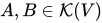
A
,
B
∈
K
(
V
)
{\displaystyle A,B\in {\mathcal {K}}(V)}
vol
(
∙
+
A
)
∗
vol
(
∙
+
B
)
=
vol
(
∙
+
A
+
B
)
.
{\displaystyle \operatorname {vol} (\bullet +A)\ast \operatorname {vol} (\bullet +B)=\operatorname {vol} (\bullet +A+B).}
Val
∞
(
V
)
×
Val
∞
(
V
)
→
Val
∞
(
V
)
,
{\displaystyle \operatorname {Val} ^{\infty }(V)\times \operatorname {Val} ^{\infty }(V)\to \operatorname {Val} ^{\infty }(V),}
ϕ
∈
Val
n
−
i
∞
(
V
)
,
{\displaystyle \phi \in \operatorname {Val} _{n-i}^{\infty }(V),}
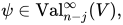
ψ
∈
Val
n
−
j
∞
(
V
)
,
{\displaystyle \psi \in \operatorname {Val} _{n-j}^{\infty }(V),}
ϕ
∗
ψ
∈
Val
n
−
i
−
j
∞
(
V
)
.
{\displaystyle \phi \ast \psi \in \operatorname {Val} _{n-i-j}^{\infty }(V).}
例えば、 凸体の混合体積を とします。 滑らかな境界と厳密に正のガウス曲率を持つ
凸 体が固定されている場合、 次
数の滑らかな評価を定義します。 このような2つの評価の畳み込みは、
のみ に依存する定数です。
V
(
K
1
,
…
,
K
n
)
{\displaystyle V(K_{1},\ldots ,K_{n})}
K
1
,
…
,
K
n
⊂
R
n
.
{\displaystyle K_{1},\ldots ,K_{n}\subset \mathbb {R} ^{n}.}
A
1
,
…
,
A
n
−
i
{\displaystyle A_{1},\dots ,A_{n-i}}
R
n
{\displaystyle \mathbb {R} ^{n}}
ϕ
(
K
)
=
V
(
K
[
i
]
,
A
1
,
…
,
A
n
−
i
)
{\displaystyle \phi (K)=V(K[i],A_{1},\dots ,A_{n-i})}
i
.
{\displaystyle i.}
V
(
∙
[
i
]
,
A
1
,
…
,
A
n
−
i
)
∗
V
(
∙
[
j
]
,
B
1
,
…
,
B
n
−
j
)
=
c
i
,
j
V
(
∙
[
n
−
j
−
i
]
,
A
1
,
…
,
A
n
−
i
,
B
1
,
…
,
B
n
−
j
)
,
{\displaystyle V(\bullet [i],A_{1},\dots ,A_{n-i})\ast V(\bullet [j],B_{1},\dots ,B_{n-j})=c_{i,j}V(\bullet [n-j-i],A_{1},\dots ,A_{n-i},B_{1},\dots ,B_{n-j}),}
c
i
,
j
{\displaystyle c_{i,j}}
i
,
j
,
n
.
{\displaystyle i,j,n.}
アレスカー・フーリエ変換は、アレスカーによって発見された 複素数値の自然な -同変同型
であり 、その名前の由来となっている古典的なフーリエ変換に似た多くの特性を備えています。
G
L
(
V
)
{\displaystyle GL(V)}
F
:
Val
∞
(
V
)
→
Val
∞
(
V
∗
)
⊗
Dens
(
V
)
,
{\displaystyle \mathbb {F} :\operatorname {Val} ^{\infty }(V)\to \operatorname {Val} ^{\infty }(V^{*})\otimes \operatorname {Dens} (V),}
つまり、グレーディングを逆にして 、積と畳み込みを絡み合わせます。
F
:
Val
k
∞
(
V
)
→
Val
n
−
k
∞
(
V
∗
)
⊗
Dens
(
V
)
,
{\displaystyle \mathbb {F} :\operatorname {Val} _{k}^{\infty }(V)\to \operatorname {Val} _{n-k}^{\infty }(V^{*})\otimes \operatorname {Dens} (V),}
F
(
ϕ
⋅
ψ
)
=
F
ϕ
∗
F
ψ
.
{\displaystyle \mathbb {F} (\phi \cdot \psi )=\mathbb {F} \phi \ast \mathbb {F} \psi .}
簡単にするためにユークリッド構造を固定して識別すると、次の 恒等式が得られます 。偶数値の場合、クレイン埋め込みの観点からフーリエ変換を簡単に記述できます。 特に、実数値の偶数値は、フーリエ変換後も実数値のままです。
V
=
V
∗
,
{\displaystyle V=V^{*},}
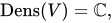
Dens
(
V
)
=
C
,
{\displaystyle \operatorname {Dens} (V)=\mathbb {C} ,}
F
2
ϕ
(
K
)
=
ϕ
(
−
K
)
.
{\displaystyle \mathbb {F} ^{2}\phi (K)=\phi (-K).}
Kl
F
ϕ
(
E
)
=
Kl
ϕ
(
E
⊥
)
.
{\displaystyle \operatorname {Kl} _{\mathbb {F} \phi }(E)=\operatorname {Kl} _{\phi }(E^{\perp }).}
奇数値の場合、フーリエ変換の記述は実質的により複雑になります。偶数値の場合とは異なり、純粋に幾何学的な性質を持つものではなくなります。たとえば、実数値の奇数値の空間は保存されません。
引き戻しと押し進め 線形写像が与えられた場合、プルバック とプッシュフォワード という誘導された操作があります。 プルバックは 2 つのうちより単純で、次のように表されます。 明らかに、評価のパリティと同次性を維持します。 が単射でない
場合、プルバックは滑らかさを維持しないことに注意してください。
f
:
U
→
V
,
{\displaystyle f:U\to V,}
f
∗
:
Val
(
V
)
→
Val
(
U
)
{\displaystyle f^{*}:\operatorname {Val} (V)\to \operatorname {Val} (U)}
f
∗
:
Val
(
U
)
⊗
Dens
(
U
)
∗
→
Val
(
V
)
⊗
Dens
(
V
)
∗
.
{\displaystyle f_{*}:\operatorname {Val} (U)\otimes \operatorname {Dens} (U)^{*}\to \operatorname {Val} (V)\otimes \operatorname {Dens} (V)^{*}.}
f
∗
ϕ
(
K
)
=
ϕ
(
f
(
K
)
)
.
{\displaystyle f^{*}\phi (K)=\phi (f(K)).}
f
{\displaystyle f}
プッシュフォワードを形式的に定義するのは困難です。簡単にするために、 および上のルベーグ測度を固定します。プッシュフォワードは、 すべてのに対して 形式の付値への作用を記述することによって一意に特徴付けることができ、 その後
、既約定理を使用してすべての付値への連続性によって拡張されます。全射写像の場合、 包含の場合、 分割を選択します。
非公式には、プッシュフォワードは、アレスカー-ポアンカレペアリングに関してプルバックの双対です。 およびに対して。ただし、この恒等式は、ペアリングが滑らかな付値に対してのみ明確に定義されているため、注意深く解釈する必要があります。詳細については、 [7]を
参照してください。
U
{\displaystyle U}
V
.
{\displaystyle V.}
vol
(
∙
+
A
)
,
{\displaystyle \operatorname {vol} (\bullet +A),}
A
∈
K
(
U
)
,
{\displaystyle A\in {\mathcal {K}}(U),}
f
,
{\displaystyle f,}
f
∗
vol
(
∙
+
A
)
=
vol
(
∙
+
f
(
A
)
)
.
{\displaystyle f_{*}\operatorname {vol} (\bullet +A)=\operatorname {vol} (\bullet +f(A)).}
f
:
U
↪
V
,
{\displaystyle f:U\hookrightarrow V,}
V
=
U
⊕
W
.
{\displaystyle V=U\oplus W.}
f
∗
vol
(
∙
+
A
)
(
K
)
=
∫
W
vol
(
K
∩
(
U
+
w
)
+
A
)
d
w
.
{\displaystyle f_{*}\operatorname {vol} (\bullet +A)(K)=\int _{W}\operatorname {vol} (K\cap (U+w)+A)dw.}
ϕ
∈
Val
(
V
)
{\displaystyle \phi \in \operatorname {Val} (V)}
ψ
∈
Val
(
U
)
⊗
Dens
(
U
)
∗
,
{\displaystyle \psi \in \operatorname {Val} (U)\otimes \operatorname {Dens} (U)^{*},}
⟨
f
∗
ϕ
,
ψ
⟩
=
⟨
ϕ
,
f
∗
ψ
⟩
.
{\displaystyle \langle f^{*}\phi ,\psi \rangle =\langle \phi ,f_{*}\psi \rangle .}
多様体上の評価 2006年に始まった一連の論文で、アレスカーは凸体上の付値理論を拡張した多様体上の付値理論の基礎を築いた。この拡張につながる重要な観察は、通常のサイクル( 1 )上の積分により、凸集合よりもはるかに一般的な集合上で滑らかな並進不変の付値を評価できるということである。また、( 1 )は、形式が並進不変であるという要件を削除し、並進不変ルベーグ測度を任意の滑らかな測度に置き換えることによって、一般的な滑らかな付値を定義することを示唆している 。
ω
{\displaystyle \omega }
をn次元の滑らかな多様体とし、を の共球面束、つまり余接束の有向射影化とします 。 を の コンパクト な微分可能多面体の集合とします。 の 外向き共法線からなる の 法線サイクルは、 当然 次元のリプシッツ部分多様体です。
X
{\displaystyle X}
P
X
=
P
+
(
T
∗
X
)
{\displaystyle \mathbb {P} _{X}=\mathbb {P} _{+}(T^{*}X)}
X
,
{\displaystyle X,}
P
(
X
)
{\displaystyle {\mathcal {P}}(X)}
X
.
{\displaystyle X.}
N
(
A
)
⊂
P
X
{\displaystyle N(A)\subset \mathbb {P} _{X}}
A
∈
P
(
X
)
,
{\displaystyle A\in {\mathcal {P}}(X),}
A
,
{\displaystyle A,}
n
−
1.
{\displaystyle n-1.}
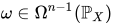
提示を簡単にするために、我々は が有向であると仮定する が、実際には滑らかな値の概念は有向性に依存しない。 上の滑らかな値の空間は の 形の
関数から成り、
ここで と は任意である。 の開部分集合上の滑らかな値は 上のソフト層を形成する ことがアレスカーによって示された。
X
{\displaystyle X}
V
∞
(
X
)
{\displaystyle {\mathcal {V}}^{\infty }(X)}
X
{\displaystyle X}
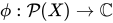
ϕ
:
P
(
X
)
→
C
{\displaystyle \phi :{\mathcal {P}}(X)\to \mathbb {C} }
ϕ
(
A
)
=
∫
A
μ
+
∫
N
(
A
)
ω
,
A
∈
P
(
X
)
,
{\displaystyle \phi (A)=\int _{A}\mu +\int _{N(A)}\omega ,\qquad A\in {\mathcal {P}}(X),}
μ
∈
Ω
n
(
X
)
{\displaystyle \mu \in \Omega ^{n}(X)}
ω
∈
Ω
n
−
1
(
P
X
)
{\displaystyle \omega \in \Omega ^{n-1}(\mathbb {P} _{X})}
X
{\displaystyle X}
X
.
{\displaystyle X.}
例 以下は滑らかな多様体上の滑らかな評価の例です 。
X
{\displaystyle X}
スムーズな対策
X
.
{\displaystyle X.}
オイラー 特性は、 ガウス ・ボネ定理 に関するチャーン [8] の研究から導かれ 、オイラー特性を表すためにこのような および が構築されました。特に、 は チャーン・ガウス・ボネ積分関数 であり、リーマン曲率テンソルのパフィアンです。
μ
{\displaystyle \mu }
ω
{\displaystyle \omega }
μ
{\displaystyle \mu }
がリーマンである場合 、リプシッツ・キリング評価または固有体積は 滑らかな評価です。が ユークリッド空間への 等長浸漬で ある場合、 は 上の通常の固有体積を表します (引き戻しの定義については以下を参照)。これらの評価の存在は、ワイルのチューブ公式の本質です。 [9]
X
{\displaystyle X}
V
0
X
=
χ
,
V
1
X
,
…
,
V
n
X
=
v
o
l
X
{\displaystyle V_{0}^{X}=\chi ,V_{1}^{X},\ldots ,V_{n}^{X}=\mathrm {vol} _{X}}
f
:
X
→
R
m
{\displaystyle f:X\to \mathbb {R} ^{m}}
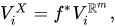
V
i
X
=
f
∗
V
i
R
m
,
{\displaystyle V_{i}^{X}=f^{*}V_{i}^{\mathbb {R} ^{m}},}
V
i
R
m
{\displaystyle V_{i}^{\mathbb {R} ^{m}}}
R
m
{\displaystyle \mathbb {R} ^{m}}
を 複素射影空間 とし 、を 固定次元のすべての複素射影部分空間のグラスマン多様体とすると、 関数
C
P
n
{\displaystyle \mathbb {C} P^{n}}
G
r
k
C
{\displaystyle \mathrm {Gr} _{k}^{\mathbb {C} }}
k
.
{\displaystyle k.}
ϕ
(
A
)
=
∫
G
r
k
C
χ
(
A
∩
E
)
d
E
,
A
∈
P
(
C
P
n
)
,
{\displaystyle \phi (A)=\int _{\mathrm {Gr} _{k}^{\mathbb {C} }}\chi (A\cap E)dE,\qquad A\in {\mathcal {P}}(\mathbb {C} P^{n}),}
ここで積分はハール確率測度に関して なめらかな評価である。これはFuの研究から導かれる。 [10]
G
r
k
C
,
{\displaystyle \mathrm {Gr} _{k}^{\mathbb {C} },}
濾過 空間は 一般に自然な段階分けを許さないが、標準的なフィルタリングを実行する。
ここでは、 上の滑らかな測度で構成され 、 によって生成されるイデアルの 形式で与えられる。 は 標準的な射影である。
V
∞
(
X
)
{\displaystyle {\mathcal {V}}^{\infty }(X)}
V
∞
(
X
)
=
W
0
⊃
W
1
⊃
⋯
⊃
W
n
.
{\displaystyle {\mathcal {V}}^{\infty }(X)=W_{0}\supset W_{1}\supset \cdots \supset W_{n}.}
W
n
{\displaystyle W_{n}}
X
,
{\displaystyle X,}
W
j
{\displaystyle W_{j}}
ω
{\displaystyle \omega }
π
∗
Ω
j
(
X
)
,
{\displaystyle \pi ^{*}\Omega ^{j}(X),}
π
:
P
X
→
X
{\displaystyle \pi :\mathbb {P} _{X}\to X}
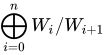
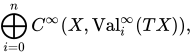
関連する次数付きベクトル空間は 、 点上のファイバーが 接空間上の同次滑らかな並進不変値 空間と なるような ベクトル束を表す 滑らかな切断空間と正準同型である。
⨁
i
=
0
n
W
i
/
W
i
+
1
{\displaystyle \bigoplus _{i=0}^{n}W_{i}/W_{i+1}}
⨁
i
=
0
n
C
∞
(
X
,
Val
i
∞
(
T
X
)
)
,
{\displaystyle \bigoplus _{i=0}^{n}C^{\infty }(X,\operatorname {Val} _{i}^{\infty }(TX)),}
Val
i
∞
(
T
X
)
{\displaystyle \operatorname {Val} _{i}^{\infty }(TX)}
X
{\displaystyle X}
x
∈
X
{\displaystyle x\in X}
Val
i
∞
(
T
x
X
)
,
{\displaystyle \operatorname {Val} _{i}^{\infty }(T_{x}X),}
i
{\displaystyle i}
T
x
X
.
{\displaystyle T_{x}X.}
製品 この空間は 自然積を許容します。この積は連続、可換、結合的であり、濾過と互換性
があり、恒等元としてオイラー特性を持ちます。また、埋め込み部分多様体への制限と可換であり、微分同相群は代数自己同型によって 作用します 。
V
∞
(
X
)
{\displaystyle {\mathcal {V}}^{\infty }(X)}
W
i
⋅
W
j
⊂
W
i
+
j
,
{\displaystyle W_{i}\cdot W_{j}\subset W_{i+j},}
X
{\displaystyle X}
V
∞
(
X
)
{\displaystyle {\mathcal {V}}^{\infty }(X)}
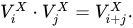
例えば、 がリーマン分布である場合、リプシッツ・キリング評価は
X
{\displaystyle X}
V
i
X
⋅
V
j
X
=
V
i
+
j
X
.
{\displaystyle V_{i}^{X}\cdot V_{j}^{X}=V_{i+j}^{X}.}
アレスカー-ポアンカレ双対性は依然として有効です。コンパクトの場合、 ペアリングは非退化であると言えます 。並進不変の場合と同様に、この双対性を使用して一般化された評価を定義できます。並進不変の場合とは異なり、多様体上の評価については連続的な評価の適切な定義は存在しません。
X
{\displaystyle X}
V
∞
(
X
)
×
V
∞
(
X
)
→
C
,
{\displaystyle {\mathcal {V}}^{\infty }(X)\times {\mathcal {V}}^{\infty }(X)\to \mathbb {C} ,}
(
ϕ
,
ψ
)
↦
(
ϕ
⋅
ψ
)
(
X
)
{\displaystyle (\phi ,\psi )\mapsto (\phi \cdot \psi )(X)}
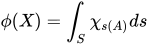
評価値の積は、部分集合の交差の幾何学的操作を厳密に反映しています。非公式には、一般化された評価値を考えます。 積は 次のように与えられます。ここで、形式の一般化された評価値を平均化することで滑らかな評価値を得ることができます。 より正確には、 が十分に大きな測定された微分同相写像族である
場合、は滑らかな評価値です。次に、次
を見てください。 [11]
χ
A
=
χ
(
A
∩
∙
)
.
{\displaystyle \chi _{A}=\chi (A\cap \bullet ).}
χ
A
⋅
χ
B
=
χ
A
∩
B
.
{\displaystyle \chi _{A}\cdot \chi _{B}=\chi _{A\cap B}.}
χ
A
,
{\displaystyle \chi _{A},}
ϕ
(
X
)
=
∫
S
χ
s
(
A
)
d
s
{\displaystyle \phi (X)=\int _{S}\chi _{s(A)}ds}
S
{\displaystyle S}
∫
S
χ
s
(
A
)
d
s
⋅
∫
S
′
χ
s
′
(
B
)
d
s
′
=
∫
S
×
S
′
χ
s
(
A
)
∩
s
′
(
B
)
d
s
d
s
′
,
{\displaystyle \int _{S}\chi _{s(A)}ds\cdot \int _{S'}\chi _{s'(B)}ds'=\int _{S\times S'}\chi _{s(A)\cap s'(B)}dsds',}
引き戻しと押し進め 滑らかな多様体の滑らか な浸漬はすべて、プルバック マップを誘導します。 が埋め込みである場合、
プルバック
はフィルターされた代数の射です。 滑らかな適切な浸漬はすべて、次のように プッシュフォワード マップを定義します。 プッシュフォワード は
、 フィルターとも互換性があります。
一般的な滑らかなマップの場合、いくつかの制限の下で、一般化された評価に対してプルバックとプッシュフォワードを定義できます。
f
:
X
→
Y
{\displaystyle f:X\to Y}
f
∗
:
V
∞
(
Y
)
→
V
∞
(
X
)
.
{\displaystyle f^{*}:{\mathcal {V}}^{\infty }(Y)\to {\mathcal {V}}^{\infty }(X).}
f
{\displaystyle f}
(
f
∗
ϕ
)
(
A
)
=
ϕ
(
f
(
A
)
)
,
A
∈
P
(
X
)
.
{\displaystyle (f^{*}\phi )(A)=\phi (f(A)),\qquad A\in {\mathcal {P}}(X).}
f
:
X
→
Y
{\displaystyle f:X\to Y}
f
∗
:
V
∞
(
X
)
→
V
∞
(
Y
)
{\displaystyle f^{*}:{\mathcal {V}}^{\infty }(X)\to {\mathcal {V}}^{\infty }(Y)}
(
f
∗
ϕ
)
(
A
)
=
ϕ
(
f
−
1
(
A
)
)
,
A
∈
P
(
Y
)
.
{\displaystyle (f_{*}\phi )(A)=\phi (f^{-1}(A)),\qquad A\in {\mathcal {P}}(Y).}
f
∗
:
W
i
(
X
)
→
W
i
−
(
dim
X
−
dim
Y
)
(
Y
)
.
{\displaystyle f_{*}:W_{i}(X)\to W_{i-(\dim X-\dim Y)}(Y).}
積分幾何学への応用
を リーマン多様体 と し、を 球面束上で推移的に作用する の等長写像のリー群とします。これらの仮定の下で、 上の - 不変な滑らかな値 の 空間は 有限次元です。を 基底とします。 を の微分可能な多面体とします。 すると、 の形式の積分は 、 および に独立な 係数を持つ の線形結合として表すことができます 。
M
{\displaystyle M}
G
{\displaystyle G}
M
{\displaystyle M}
S
M
.
{\displaystyle SM.}
V
∞
(
M
)
G
{\displaystyle {\mathcal {V}}^{\infty }(M)^{G}}
G
{\displaystyle G}
M
{\displaystyle M}
ϕ
1
,
…
,
ϕ
m
{\displaystyle \phi _{1},\ldots ,\phi _{m}}
A
,
B
∈
P
(
M
)
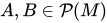
{\displaystyle A,B\in {\mathcal {P}}(M)}
M
.
{\displaystyle M.}
∫
G
ϕ
i
(
A
∩
g
B
)
d
g
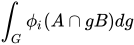
{\displaystyle \int _{G}\phi _{i}(A\cap gB)dg}
ϕ
k
(
A
)
ϕ
l
(
B
)
{\displaystyle \phi _{k}(A)\phi _{l}(B)}
c
i
k
l
{\displaystyle c_{i}^{kl}}
A
{\displaystyle A}
B
{\displaystyle B}
このタイプの式は運動学的公式 と呼ばれます 。この一般性におけるその存在はフーによって証明されました。 [10] 3つの単連結な実空間形式、つまり球面、ユークリッド空間、双曲空間については、 ブラシュケ 、 サンタロ 、 チャーン 、 フェデラー に遡ります 。
運動学的公式を明示的に記述することは、典型的には困難な問題である。実際、実空間形式から複素空間形式へのステップで既に相当な困難が生じており、これらは最近になってようやく Bernig、Fu、Solanes によって解決された。 [12] [13] この進歩の原因となった重要な洞察は、運動学的公式が不変値の代数と同じ情報を含んでいるということである
。正確な記述のために、 を
運動学的演算子、つまり運動学的公式 ( 2 ) によって決定されるマップとします。
を線形同型である Alesker-Poincaré 双対性を表すものとします。最後に、 を積マップの随伴とします。 積分幾何学への値の操作を関連付ける代数積分幾何学の基本定理は、 ポアンカレ双対性を使用して と同一視する場合、 と述べ て いる 。
V
∞
(
M
)
G
.
{\displaystyle {\mathcal {V}}^{\infty }(M)^{G}.}
k
G
:
V
∞
(
M
)
G
→
V
∞
(
M
)
G
⊗
V
∞
(
M
)
G
{\displaystyle k_{G}:{\mathcal {V}}^{\infty }(M)^{G}\to {\mathcal {V}}^{\infty }(M)^{G}\otimes {\mathcal {V}}^{\infty }(M)^{G}}
pd
:
V
∞
(
M
)
G
→
V
∞
(
M
)
G
∗
{\displaystyle \operatorname {pd} :{\mathcal {V}}^{\infty }(M)^{G}\to {\mathcal {V}}^{\infty }(M)^{G*}}
m
G
∗
{\displaystyle m_{G}^{*}}
m
G
:
V
∞
(
M
)
G
⊗
V
∞
(
M
)
G
→
V
∞
(
M
)
G
.
{\displaystyle m_{G}:{\mathcal {V}}^{\infty }(M)^{G}\otimes {\mathcal {V}}^{\infty }(M)^{G}\to {\mathcal {V}}^{\infty }(M)^{G}.}
V
∞
(
M
)
G
{\displaystyle {\mathcal {V}}^{\infty }(M)^{G}}
V
∞
(
M
)
G
∗
,
{\displaystyle {\mathcal {V}}^{\infty }(M)^{G*},}
k
G
=
m
G
∗
{\displaystyle k_{G}=m_{G}^{*}}
。
参照 ハドヴィガーの定理 – 積分幾何学における定理 積分幾何学 – その空間の対称群の下での幾何学的空間不変量上の測度の理論 Pages displaying wikidata descriptions as a fallback 混合ボリューム モジュラーセット関数 – マッピング関数 Pages displaying short descriptions of redirect targets 集合関数 – 集合から数値への関数 評価(測度論) - 測度論または領域理論におけるマップ Pages displaying wikidata descriptions as a fallback
参考文献
^ マクマレン、ピーター (1980)、「コンパクト凸集合の空間における連続並進不変評価」、 Archiv der Mathematik 、 34 (4):377–384、 doi :10.1007 / BF01224974、 S2CID 122127897 ^ ab Hadwiger、Hugo (1957)、 Vorlesungen über Inhalt、Oberfläche und Isoperimetrie 、Die Grundlehren der Mathematischen Wissenschaften、vol. 93、ベルリン-ゲッティンゲン-ハイデルベルク: Springer-Verlag、 doi :10.1007/978-3-642-94702-5、 ISBN 978-3-642-94703-2 ^ ab Schneider, Rolf (1996)、「凸体の単純評価」、 Mathematika 、 43 (1): 32–39、 doi :10.1112/S0025579300011578 ^ クレイン、ダニエル A. (1995)、「ハドヴィガーの特徴づけ定理の簡単な証明」、 Mathematika 、 42 (2): 329–339、 doi :10.1112/S0025579300014625 ^ ab Alesker, Semyon (2018)、 評価理論入門 、CBMS数学地域会議シリーズ、第126巻、プロビデンス、ロードアイランド州:アメリカ数学会 ^ Alesker, Semyon (2001)、「P. McMullen の予想の解決を伴う凸集合上の変換不変値の説明」、 幾何学および機能解析 、 11 (2): 244–272、 doi :10.1007/PL00001675、 S2CID 122986474 ^ Alesker, Semyon (2011)、「凸集合上の変換不変値に対するフーリエ型変換」、 Israel Journal of Mathematics 、 181 : 189–294、 arXiv : math/0702842 、 doi : 10.1007/s11856-011-0008-6 ^ Chern, Shiing-Shen (1945)、「リーマン多様体の曲率積分について」、 Annals of Mathematics 、第 2 シリーズ、 46 (4): 674–684、 doi :10.2307/1969203、 JSTOR 1969203、 S2CID 123348816 ^ ワイル、ヘルマン (1939)、「チューブの体積について」、 アメリカ数学誌 、 61 (2): 461–472、 doi :10.2307/2371513、 JSTOR 2371513 ^ ab Fu, Joseph HG (1990)、「積分幾何学における運動学的公式」、 インディアナ大学数学ジャーナル 、 39 (4): 1115–1154、 doi : 10.1512/iumj.1990.39.39052 ^ Fu, Joseph HG (2016)、「交差理論とアレスカー積」、 インディアナ大学数学ジャーナル 、 65 (4): 1347–1371、 arXiv : 1408.4106 、 doi :10.1512/iumj.2016.65.5846、 S2CID 119736489 ^ ベルニグ、アンドレアス; フー、ジョセフHG; ソラネス、ギル(2014)、「複素空間形式の積分幾何学」、 幾何学的および機能的分析 、 24 (2):403–49、 arXiv : 1204.0604 、 doi : 10.1007 / s00039-014-0251-1 2 ^ ベルニグ、アンドレアス; フー、ジョセフ HG (2011)、「エルミート積分幾何学」、 数学年報 、第 2 シリーズ、 173 (2): 907–945、 arXiv : 0801.0711 、 doi : 10.4007/annals.2011.173.2.7
文献 S. Alesker (2018)。 評価理論入門 。CBMS 数学地域会議シリーズ、126。アメリカ数学会、プロビデンス、ロードアイランド州 。ISBN 978-1-4704-4359-7 。 S. Alesker 、JHG Fu (2014)。 積分幾何学と評価 。数学上級コース。CRM Barcelona。Birkhäuser/Springer、バーゼル 。ISBN 978-1-4704-4359-7 。 DA クレイン。 G.-C.ロタ (1997)。 幾何学的確率の紹介 。レツィオーニ・リンセ。 【リンセイ講座】。ケンブリッジ大学出版局。 ISBN 0-521-59362-X 。 R. シュナイダー (2014)。 凸体: ブルン・ミンコフスキー理論 。数学とその応用百科事典、151。ケンブリッジ大学出版局、ケンブリッジ、ロードアイランド州 。ISBN 978-1-107-60101-7 。 





















































































![{\displaystyle \phi (K)=V(K[i],A_{1},\dots ,A_{ni})}](https://wikimedia.org/api/rest_v1/media/math/render/svg/6516b4c8970c0f605545a30991eaf8190501dd05)
![{\displaystyle V(\bullet [i],A_{1},\dots ,A_{ni})\ast V(\bullet [j],B_{1},\dots ,B_{nj})=c_{i,j}V(\bullet [nji],A_{1},\dots ,A_{ni},B_{1},\dots ,B_{nj}),}](https://wikimedia.org/api/rest_v1/media/math/render/svg/dd25e09999542c2d0af725694dcea8ffa3fdd506)































































 。
。