熱力学量の偏微分を含む方程式
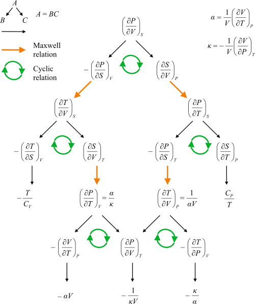
マクスウェル関係式間の経路を示すフローチャート。圧力、 温度、 体積、 エントロピー、 熱膨張係数 、 圧縮率 、 定積 熱容量 、定圧熱容量 です。
P
{\displaystyle P}
T
{\displaystyle T}
V
{\displaystyle V}
S
{\displaystyle S}
α
{\displaystyle \alpha }
κ
{\displaystyle \kappa }
C
V
{\displaystyle C_{V}}
C
P
{\displaystyle C_{P}}
マクスウェルの関係式は、 2 次導関数の対称性と 熱力学的ポテンシャル の定義から 導出できる 熱力学 の方程式の集合です。この関係式は、19 世紀の物理学者 ジェームズ・クラーク・マクスウェル にちなんで名付けられました 。
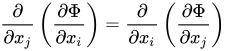
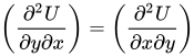
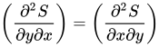
方程式 マクスウェル関係式の構造は、連続関数の2次導関数間の等式を記述したものである。これは、 2変数の 解析関数の微分順序は無関係であるという事実から直接導かれる( シュワルツの定理 )。マクスウェル関係式の場合、対象とする関数は熱力学的ポテンシャルであり、 と はそのポテンシャルの 2つの異なる 自然変数 であるため、
x
i
{\displaystyle x_{i}}
x
j
{\displaystyle x_{j}}
シュワルツの定理(一般)
∂
∂
x
j
(
∂
Φ
∂
x
i
)
=
∂
∂
x
i
(
∂
Φ
∂
x
j
)
{\displaystyle {\frac {\partial }{\partial x_{j}}}\left({\frac {\partial \Phi }{\partial x_{i}}}\right)={\frac {\partial }{\partial x_{i}}}\left({\frac {\partial \Phi }{\partial x_{j}}}\right)}
ここで、 偏導関数は 他のすべての自然変数を一定に保った状態で取られます。すべての熱力学的ポテンシャルに対して、そのポテンシャルの自然変数の数 であるマクスウェル関係式が考えられます 。
1
2
n
(
n
−
1
)
{\textstyle {\frac {1}{2}}n(n-1)}
n
{\displaystyle n}
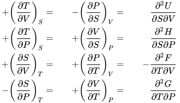
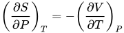
最も一般的な4つのマクスウェル関係 最も一般的な 4 つのマクスウェル関係式は、4 つの熱力学的ポテンシャルのそれぞれについて、熱的自然変数 ( 温度 、または エントロピー ) と 機械的 自然変数 ( 圧力 、または 体積 ) に関する 2 次導関数の等式です。
T
{\displaystyle T}
S
{\displaystyle S}
P
{\displaystyle P}
V
{\displaystyle V}
マクスウェルの関係 (共通)
+
(
∂
T
∂
V
)
S
=
−
(
∂
P
∂
S
)
V
=
∂
2
U
∂
S
∂
V
+
(
∂
T
∂
P
)
S
=
+
(
∂
V
∂
S
)
P
=
∂
2
H
∂
S
∂
P
+
(
∂
S
∂
V
)
T
=
+
(
∂
P
∂
T
)
V
=
−
∂
2
F
∂
T
∂
V
−
(
∂
S
∂
P
)
T
=
+
(
∂
V
∂
T
)
P
=
∂
2
G
∂
T
∂
P
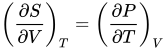
{\displaystyle {\begin{aligned}+\left({\frac {\partial T}{\partial V}}\right)_{S}&=&-\left({\frac {\partial P}{\partial S}}\right)_{V}&=&{\frac {\partial ^{2}U}{\partial S\partial V}}\\+\left({\frac {\partial T}{\partial P}}\right)_{S}&=&+\left({\frac {\partial V}{\partial S}}\right)_{P}&=&{\frac {\partial ^{2}H}{\partial S\partial P}}\\+\left({\frac {\partial S}{\partial V}}\right)_{T}&=&+\left({\frac {\partial P}{\partial T}}\right)_{V}&=&-{\frac {\partial ^{2}F}{\partial T\partial V}}\\-\left({\frac {\partial S}{\partial P}}\right)_{T}&=&+\left({\frac {\partial V}{\partial T}}\right)_{P}&=&{\frac {\partial ^{2}G}{\partial T\partial P}}\end{aligned}}\,\!}
ここで、自然な熱的および機械的変数の関数としてのポテンシャルは、 内部エネルギー 、 エンタルピー 、 ヘルムホルツ自由エネルギー 、および ギブス自由エネルギー です。 熱力学の四角形は、これらの関係を思い出して導くための 記憶法 として使用できます 。これらの関係の有用性は、直接測定できないエントロピーの変化を、温度、体積、圧力などの測定可能な量で定量化することにあります。
U
(
S
,
V
)
{\displaystyle U(S,V)}
H
(
S
,
P
)
{\displaystyle H(S,P)}
F
(
T
,
V
)
{\displaystyle F(T,V)}
G
(
T
,
P
)
{\displaystyle G(T,P)}
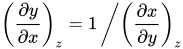
各方程式は、マクスウェル関係とも呼ばれる
関係を使用して再表現できます
。
(
∂
y
∂
x
)
z
=
1
/
(
∂
x
∂
y
)
z
{\displaystyle \left({\frac {\partial y}{\partial x}}\right)_{z}=1\left/\left({\frac {\partial x}{\partial y}}\right)_{z}\right.}
派生語
短い導出 このセクションは[1] の第5章に基づいています。
2 次元 面上を移動するように制限された 4 つの実変数 が与えられているとします 。そのうちの 2 つがわかれば、他の 2 つを一意に (一般的に) 決定できます。
(
x
,
y
,
z
,
w
)
{\displaystyle (x,y,z,w)}
C
2
{\displaystyle C^{2}}
R
4
{\displaystyle \mathbb {R} ^{4}}
特に、任意の 2 つの変数を独立変数として取り、他の 2 つを従属変数とすると、これらすべての偏微分を取ることができます。
命題:
(
∂
w
∂
y
)
z
=
(
∂
w
∂
x
)
z
(
∂
x
∂
y
)
z
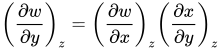
{\displaystyle \left({\frac {\partial w}{\partial y}}\right)_{z}=\left({\frac {\partial w}{\partial x}}\right)_{z}\left({\frac {\partial x}{\partial y}}\right)_{z}}
証明: これは単なる 連鎖律 です。
命題:
(
∂
x
∂
y
)
z
(
∂
y
∂
z
)
x
(
∂
z
∂
x
)
y
=
−
1
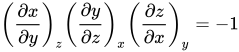
{\displaystyle \left({\frac {\partial x}{\partial y}}\right)_{z}\left({\frac {\partial y}{\partial z}}\right)_{x}\left({\frac {\partial z}{\partial x}}\right)_{y}=-1}
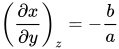
証明。 は無視できます 。すると、局所的には表面は になります 。すると 、 などになります。ここで、これらを掛け合わせます。
w
{\displaystyle w}
a
x
+
b
y
+
c
z
+
d
=
0
{\displaystyle ax+by+cz+d=0}
(
∂
x
∂
y
)
z
=
−
b
a
{\displaystyle \left({\frac {\partial x}{\partial y}}\right)_{z}=-{\frac {b}{a}}}
マクスウェルの関係式の証明:
可能な熱力学的状態の 2 次元表面上に制限された
4 つの実変数があります。これにより、前の 2 つの命題を使用できます。
(
T
,
S
,
p
,
V
)
{\displaystyle (T,S,p,V)}
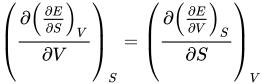
4 つの関係のうち最初の関係を証明すれば十分です。他の 3 つは、前の 2 つの命題を使用して最初の関係を変換することによって得られるからです。 を独立変数として、 を 従属変数として選択します。 となります
。
V
,
S
{\displaystyle V,S}
E
{\displaystyle E}
d
E
=
−
p
d
V
+
T
d
S
{\displaystyle dE=-pdV+TdS}
ここで、 表面は 、つまり なので、 結果は となります。
∂
V
,
S
E
=
∂
S
,
V
E
{\displaystyle \partial _{V,S}E=\partial _{S,V}E}
C
2
{\displaystyle C^{2}}
(
∂
(
∂
E
∂
S
)
V
∂
V
)
S
=
(
∂
(
∂
E
∂
V
)
S
∂
S
)
V
{\displaystyle \left({\frac {\partial \left({\frac {\partial E}{\partial S}}\right)_{V}}{\partial V}}\right)_{S}=\left({\frac {\partial \left({\frac {\partial E}{\partial V}}\right)_{S}}{\partial S}}\right)_{V}}
別の派生 に基づく。 [2]
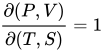
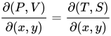
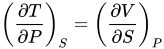
なので 、任意のサイクルの周りではとなります。 サイクルを無限小に取ると となります 。つまり、マップは面積保存です。ヤコビアンの連鎖律により、任意の座標変換 に対して と なります。 ここで をさまざまな値に設定すると 、4つのマクスウェル関係式が得られます。たとえば、 を設定すると、次のようになります。
d
U
=
T
d
S
−
P
d
V
{\displaystyle dU=TdS-PdV}
0
=
∮
d
U
=
∮
T
d
S
−
∮
P
d
V
{\displaystyle 0=\oint dU=\oint TdS-\oint PdV}
∂
(
P
,
V
)
∂
(
T
,
S
)
=
1
{\displaystyle {\frac {\partial (P,V)}{\partial (T,S)}}=1}
(
x
,
y
)
{\displaystyle (x,y)}
∂
(
P
,
V
)
∂
(
x
,
y
)
=
∂
(
T
,
S
)
∂
(
x
,
y
)
{\displaystyle {\frac {\partial (P,V)}{\partial (x,y)}}={\frac {\partial (T,S)}{\partial (x,y)}}}
(
x
,
y
)
{\displaystyle (x,y)}
(
x
,
y
)
=
(
P
,
S
)
{\displaystyle (x,y)=(P,S)}
(
∂
T
∂
P
)
S
=
(
∂
V
∂
S
)
P
{\displaystyle \left({\frac {\partial T}{\partial P}}\right)_{S}=\left({\frac {\partial V}{\partial S}}\right)_{P}}
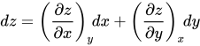
拡張導出 マクスウェル関係は、単純な偏微分規則、特に 関数の全微分 と 2 次偏微分を評価する対称性に基づいています。
導出 マクスウェルの関係式の導出は、 熱力学ポテンシャル の微分形式から演繹できます。内部エネルギー U
の微分形式 は、
この式は 、形式の
全微分 に似ています。形式の任意の方程式について、
次
の式が示されることがわかります
。
方程式 を考えてみましょ う。これで、次の式がすぐにわかります。また、
連続する2次導関数を持つ関数については、混合偏導関数が同一であることもわかっているため ( 2次導関数の対称性 )、つまり
、次の式
が成り立ちます。したがって、次の式が成り立ち、したがって、次の式が成り立ちます
。
d
U
=
T
d
S
−
P
d
V
{\displaystyle dU=T\,dS-P\,dV}
d
z
=
(
∂
z
∂
x
)
y
d
x
+
(
∂
z
∂
y
)
x
d
y
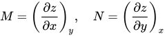
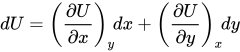
{\displaystyle dz=\left({\frac {\partial z}{\partial x}}\right)_{y}\!dx+\left({\frac {\partial z}{\partial y}}\right)_{x}\!dy}
d
z
=
M
d
x
+
N
d
y
{\displaystyle dz=M\,dx+N\,dy}
M
=
(
∂
z
∂
x
)
y
,
N
=
(
∂
z
∂
y
)
x
{\displaystyle M=\left({\frac {\partial z}{\partial x}}\right)_{y},\quad N=\left({\frac {\partial z}{\partial y}}\right)_{x}}
d
U
=
T
d
S
−
P
d
V
{\displaystyle dU=T\,dS-P\,dV}
T
=
(
∂
U
∂
S
)
V
,
−
P
=
(
∂
U
∂
V
)
S
{\displaystyle T=\left({\frac {\partial U}{\partial S}}\right)_{V},\quad -P=\left({\frac {\partial U}{\partial V}}\right)_{S}}
∂
∂
y
(
∂
z
∂
x
)
y
=
∂
∂
x
(
∂
z
∂
y
)
x
=
∂
2
z
∂
y
∂
x
=
∂
2
z
∂
x
∂
y
{\displaystyle {\frac {\partial }{\partial y}}\left({\frac {\partial z}{\partial x}}\right)_{y}={\frac {\partial }{\partial x}}\left({\frac {\partial z}{\partial y}}\right)_{x}={\frac {\partial ^{2}z}{\partial y\partial x}}={\frac {\partial ^{2}z}{\partial x\partial y}}}
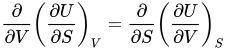
∂
∂
V
(
∂
U
∂
S
)
V
=
∂
∂
S
(
∂
U
∂
V
)
S
{\displaystyle {\frac {\partial }{\partial V}}\left({\frac {\partial U}{\partial S}}\right)_{V}={\frac {\partial }{\partial S}}\left({\frac {\partial U}{\partial V}}\right)_{S}}
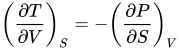
(
∂
T
∂
V
)
S
=
−
(
∂
P
∂
S
)
V
{\displaystyle \left({\frac {\partial T}{\partial V}}\right)_{S}=-\left({\frac {\partial P}{\partial S}}\right)_{V}}
ヘルムホルツ自由エネルギーからのマクスウェル関係式の導出
ヘルムホルツ自由エネルギーの微分形式は
、
2 次導関数の対称性から
次の式
が得られます。他の 2 つのマクスウェル関係式は、エンタルピーの微分形式 とギブス自由エネルギーの微分形式から 同様の方法で導出できます。したがって、上記のすべてのマクスウェル関係式は、ギブス方程式の 1 つから得られます。
d
F
=
−
S
d
T
−
P
d
V
{\displaystyle dF=-S\,dT-P\,dV}
−
S
=
(
∂
F
∂
T
)
V
,
−
P
=
(
∂
F
∂
V
)
T
{\displaystyle -S=\left({\frac {\partial F}{\partial T}}\right)_{V},\quad -P=\left({\frac {\partial F}{\partial V}}\right)_{T}}
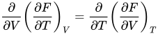
∂
∂
V
(
∂
F
∂
T
)
V
=
∂
∂
T
(
∂
F
∂
V
)
T
{\displaystyle {\frac {\partial }{\partial V}}\left({\frac {\partial F}{\partial T}}\right)_{V}={\frac {\partial }{\partial T}}\left({\frac {\partial F}{\partial V}}\right)_{T}}
(
∂
S
∂
V
)
T
=
(
∂
P
∂
T
)
V
{\displaystyle \left({\frac {\partial S}{\partial V}}\right)_{T}=\left({\frac {\partial P}{\partial T}}\right)_{V}}
d
H
=
T
d
S
+
V
d
P
{\displaystyle dH=T\,dS+V\,dP}
d
G
=
V
d
P
−
S
d
T
{\displaystyle dG=V\,dP-S\,dT}
ヤコビアンに基づく導出
熱力学の第一法則を微分形式に関する記述として 捉え
、 この式の
外微分を とる
と、 となる 。これは基本的な恒等式につながる。
d
U
=
T
d
S
−
P
d
V
{\displaystyle dU=T\,dS-P\,dV}
0
=
d
T
d
S
−
d
P
d
V
{\displaystyle 0=dT\,dS-dP\,dV}
d
(
d
U
)
=
0
{\displaystyle d(dU)=0}
d
P
d
V
=
d
T
d
S
.
{\displaystyle dP\,dV=dT\,dS.}
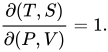
この恒等式の物理的な意味は、両辺が無限小カルノーサイクルで行われる仕事の書き方と等価であることに注目することでわかる。恒等式の書き方は次のようになる。
∂
(
T
,
S
)
∂
(
P
,
V
)
=
1.
{\displaystyle {\frac {\partial (T,S)}{\partial (P,V)}}=1.}
マクスウェルの関係は、次のように直接導かれます。例えば、
臨界ステップは最後から2番目のステップです。他のマクスウェルの関係も同様に導かれます。例えば、
(
∂
S
∂
V
)
T
=
∂
(
T
,
S
)
∂
(
T
,
V
)
=
∂
(
P
,
V
)
∂
(
T
,
V
)
=
(
∂
P
∂
T
)
V
,
{\displaystyle \left({\frac {\partial S}{\partial V}}\right)_{T}={\frac {\partial (T,S)}{\partial (T,V)}}={\frac {\partial (P,V)}{\partial (T,V)}}=\left({\frac {\partial P}{\partial T}}\right)_{V},}
(
∂
T
∂
V
)
S
=
∂
(
T
,
S
)
∂
(
V
,
S
)
=
∂
(
P
,
V
)
∂
(
V
,
S
)
=
−
(
∂
P
∂
S
)
V
.
{\displaystyle \left({\frac {\partial T}{\partial V}}\right)_{S}={\frac {\partial (T,S)}{\partial (V,S)}}={\frac {\partial (P,V)}{\partial (V,S)}}=-\left({\frac {\partial P}{\partial S}}\right)_{V}.}
マクスウェル将軍の関係 上記は、マクスウェルの関係式だけではありません。体積仕事以外の他の自然変数を含む他の仕事項を考慮したり、 粒子数を 自然変数として含めたりすると、他のマクスウェルの関係式が明らかになります。たとえば、単一成分ガスの場合、粒子数 N も上記の 4 つの熱力学的ポテンシャルの自然変数です。圧力と粒子数に関するエンタルピーのマクスウェルの関係式は次のようになります。
(
∂
μ
∂
P
)
S
,
N
=
(
∂
V
∂
N
)
S
,
P
=
∂
2
H
∂
P
∂
N
{\displaystyle \left({\frac {\partial \mu }{\partial P}}\right)_{S,N}=\left({\frac {\partial V}{\partial N}}\right)_{S,P}\qquad ={\frac {\partial ^{2}H}{\partial P\partial N}}}
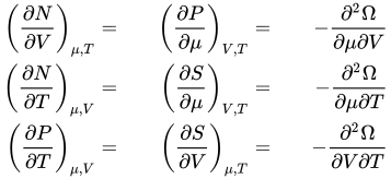
ここで、 μは 化学ポテンシャル です 。さらに、一般的に使用される 4 つのポテンシャル以外にも熱力学的ポテンシャルがあり、これらのポテンシャルのそれぞれはマクスウェル関係式のセットを生成します。たとえば、 グランドポテンシャルは 次式を生成します: [3]
Ω
(
μ
,
V
,
T
)
{\displaystyle \Omega (\mu ,V,T)}
(
∂
N
∂
V
)
μ
,
T
=
(
∂
P
∂
μ
)
V
,
T
=
−
∂
2
Ω
∂
μ
∂
V
(
∂
N
∂
T
)
μ
,
V
=
(
∂
S
∂
μ
)
V
,
T
=
−
∂
2
Ω
∂
μ
∂
T
(
∂
P
∂
T
)
μ
,
V
=
(
∂
S
∂
V
)
μ
,
T
=
−
∂
2
Ω
∂
V
∂
T
{\displaystyle {\begin{aligned}\left({\frac {\partial N}{\partial V}}\right)_{\mu ,T}&=&\left({\frac {\partial P}{\partial \mu }}\right)_{V,T}&=&-{\frac {\partial ^{2}\Omega }{\partial \mu \partial V}}\\\left({\frac {\partial N}{\partial T}}\right)_{\mu ,V}&=&\left({\frac {\partial S}{\partial \mu }}\right)_{V,T}&=&-{\frac {\partial ^{2}\Omega }{\partial \mu \partial T}}\\\left({\frac {\partial P}{\partial T}}\right)_{\mu ,V}&=&\left({\frac {\partial S}{\partial V}}\right)_{\mu ,T}&=&-{\frac {\partial ^{2}\Omega }{\partial V\partial T}}\end{aligned}}}
参照
参考文献
^ Pippard, AB (1957-01-01). 古典熱力学の要素:物理学上級者向け (第 1 版). ケンブリッジ: ケンブリッジ大学出版局. ISBN 978-0-521-09101-5 。 ^ Ritchie, David J. (2002-02-01). 「質問#78への回答。熱力学におけるマクスウェル関係についての質問」。American Journal of Physics . 70 (2): 104–104. doi :10.1119/1.1410956. ISSN 0002-9505. ^ 「熱力学ポテンシャル」 (PDF) 。 オウル大学 。 2022年12月19日時点のオリジナルより アーカイブ (PDF) 。