ホテリングのt 二乗統計量 させてΣ ^ {\displaystyle {\hat {\mathbf {\Sigma } }}} 標本共分散を 次のように定義する。
Σ ^ = 1 n − 1 ∑ 私 = 1 n ( x 私 − x ¯ ) ( x 私 − x ¯ ) ′ \displaystyle {\hat {\mathbf {\Sigma } }}={\frac {1}{n-1}}\sum _{i=1}^{n}\left(\mathbf {x} _{i}-{\overline {\mathbf {x} }}\right)\left(\mathbf {x} _{i}-{\overline {\mathbf {x} }}\right)'}
ここで、転置は アポストロフィ で表す。以下が示せる。Σ ^ {\displaystyle {\hat {\mathbf {\Sigma } }}} 正定値(半)定値 行列であり、( n − 1 ) Σ ^ {\displaystyle (n-1){\hat {\mathbf {\Sigma } }}} n − 1のp 次元ウィシャート分布 に従う。 [ 4 ] Σ ^ x ¯ = Σ ^ / n \displaystyle {\hat {\mathbf {\Sigma } }}_{\overline {\mathbf {x} }}={\hat {\mathbf {\Sigma } }}/n} 5 ]
ホテリングのt 二乗統計量 は次のように定義されます。[ 6 ]
t 2 = ( x ¯ − μ ) ′ Σ ^ x ¯ − 1 ( x ¯ − μ ) = n ( x ¯ − μ ) ′ Σ ^ − 1 ( x ¯ − μ ) 、 {\displaystyle t^{2}=({\overline {\mathbf {x} }}-{\boldsymbol {\mu }})'{\hat {\mathbf {\Sigma } }}_{\overline {\mathbf {x} }}^{-1}({\overline {\mathbf {x} }}-{\boldsymbol {\mathbf {\mu } }})=n({\overline {\mathbf {x} }}-{\boldsymbol {\mu }})'{\hat {\mathbf {\Sigma } }}^{-1}({\overline {\mathbf {x} }}-{\boldsymbol {\mathbf {\mu } }}),}
これは、標本平均と μ {\displaystyle {\boldsymbol {\mu }}} x ¯ ≈ μ \displaystyle {\overline {\mathbf {x} }}\approx {\boldsymbol {\mu }}}
分布 から、
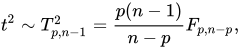
t 2 ~ T p 、 n − 1 2 = p ( n − 1 ) n − p F p 、 n − p 、 {\displaystyle t^{2}\sim T_{p,n-1}^{2}={\frac {p(n-1)}{np}}F_{p,np},}
どこF p 、 n − p {\displaystyle F_{p,np}} p とn − pを持つ F 分布
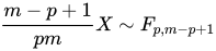
p 値p 変数とは関係ありません)、t 2 t²
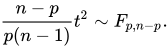
n − p p ( n − 1 ) t 2 ~ F p 、 n − p 。 \displaystyle {\frac {np}{p(n-1)}}t^{2}\sim F_{p,np}.}
次に、左辺の値を用いて、 F 分布から得られる標本に対応するp 値を算出します。同様の論理を用いて信頼区間 を求めることもできます。
モチベーション させてN p ( μ 、 Σ ) {\displaystyle {\mathcal {N}}_{p}({\boldsymbol {\mu }},{\mathbf {\Sigma } })} 位置 がp 次元正規分布μ {\displaystyle {\boldsymbol {\mu }}} 共分散 Σ \displaystyle {\mathbf {\Sigma } }}
x 1 、 … 、 x n ~ N p ( μ 、 Σ ) {\displaystyle {\mathbf {x} }_{1},\dots ,{\mathbf {x} }_{n}\sim {\mathcal {N}}_{p}({\boldsymbol {\mu }},{\mathbf {\Sigma } })}
n 個の独立同分布(iid)確率変数 であり、次のように表すことができる。p × 1 {\displaystyle p\times 1}
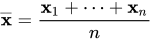
x ¯ = x 1 + ⋯ + x n n {\displaystyle {\overline {\mathbf {x} }}={\frac {\mathbf {x} _{1}+\cdots +\mathbf {x} _{n}}{n}}}
共分散を持つ標本平均 となるΣ x ¯ = Σ / n {\displaystyle {\mathbf {\Sigma } }_{\overline {\mathbf {x} }}={\mathbf {\Sigma } }/n}
( x ¯ − μ ) ′ Σ x ¯ − 1 ( x ¯ − μ ) ~ χ p 2 、 {\displaystyle ({\overline {\mathbf {x} }}-{\boldsymbol {\mu }})'{\mathbf {\Sigma } }_{\overline {\mathbf {x} }}^{-1}({\overline {\mathbf {x} }}-{\boldsymbol {\mathbf {\mu } }})\sim \chi _{p}^{2},}
どこχ p 2 {\displaystyle \chi _{p}^{2}} p のカイ二乗分布 である。 [ 7 ]
あるいは、密度関数と特性関数を用いて以下のように議論することもできる。
2標本統計量 もしx 1 、 … 、 x n x ~ N p ( μ 、 Σ ) {\displaystyle {\mathbf {x} }_{1},\dots ,{\mathbf {x} }_{n_{x}}\sim N_{p}({\boldsymbol {\mu }},{\mathbf {\Sigma } })} y 1 、 … 、 y n y ~ N p ( μ 、 Σ ) {\displaystyle {\mathbf {y} }_{1},\dots ,{\mathbf {y} }_{n_{y}}\sim N_{p}({\boldsymbol {\mu }},{\mathbf {\Sigma } })} 独立した 多変量正規分布 から独立して抽出され、次のように定義されます。
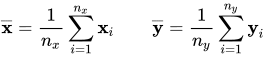
x ¯ = 1 n x ∑ 私 = 1 n x x 私 y ¯ = 1 n y ∑ 私 = 1 n y y 私 {\displaystyle {\overline {\mathbf {x} }}={\frac {1}{n_{x}}}\sum _{i=1}^{n_{x}}\mathbf {x} _{i}\qquad {\overline {\mathbf {y} }}={\frac {1}{n_{y}}}\sum _{i=1}^{n_{y}}\mathbf {y} _{i}}
サンプル平均として、
Σ ^ x = 1 n x − 1 ∑ 私 = 1 n x ( x 私 − x ¯ ) ( x 私 − x ¯ ) ′ Σ ^ y = 1 n y − 1 ∑ 私 = 1 n y ( y 私 − y ¯ ) ( y 私 − y ¯ ) ′ {\displaystyle {\begin{aligned}{\hat {\mathbf {\Sigma } }}_{\mathbf {x} }&={\frac {1}{n_{x}-1}}\sum _{i=1}^{n_{x}}\left(\mathbf {x} _{i}-{\overline {\mathbf {x} }}\right)\left(\mathbf {x} _{i}-{\overline {\mathbf {x} }}\right)'\\{\hat {\mathbf {\Sigma } }}_{\mathbf {y} }&={\frac {1}{n_{y}-1}}\sum _{i=1}^{n_{y}}\left(\mathbf {y} _{i}-{\overline {\mathbf {y} }}\right)\left(\mathbf {y} _{i}-{\overline {\mathbf {y} }}\right)'\end{aligned}}}
それぞれの標本共分散行列として。
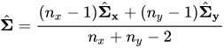
Σ ^ = ( n x − 1 ) Σ ^ x + ( n y − 1 ) Σ ^ y n x + n y − 2 {\displaystyle {\hat {\mathbf {\Sigma } }}={\frac {(n_{x}-1){\hat {\mathbf {\Sigma } }}_{\mathbf {x} }+(n_{y}-1){\hat {\mathbf {\Sigma } }}_{\mathbf {y} }}{n_{x}+n_{y}-2}}}
は、不偏なプール共分散行列推定値( プール分散 の拡張)です。
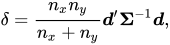
最後に、ホテリングの2標本t 二乗統計量 は
t 2 = n x n y n x + n y ( x ¯ − y ¯ ) ′ Σ ^ − 1 ( x ¯ − y ¯ ) ~ T 2 ( p 、 n x + n y − 2 ) {\displaystyle t^{2}={\frac {n_{x}n_{y}}{n_{x}+n_{y}}}({\overline {\mathbf {x} }}-{\overline {\mathbf {y} }})'{\hat {\mathbf {\Sigma } }}^{-1}({\overline {\mathbf {x} }}-{\overline {\mathbf {y} }})\sim T^{2}(p,n_{x}+n_{y}-2)}
参考文献 1 2 3 Hotelling, H. (1931). "The generalization of Student's ratio" . Annals of Mathematical Statistics 2 (3): 360– 378. doi : 10.1214/aoms/1177732979 .↑ Johnson, RA; Wichern, DW (2002). 応用多変量統計解析 . 第 5巻. Prentice Hall. ↑ エリック・W・ワイススタイン、 MathWorld 1 2 Mardia, KV; Kent, JT; Bibby, JM (1979). 多変量解析 . Academic Press. ISBN 978-0-12-471250-8 。↑ カール、フォーゲルマルク。マイケル・ロムホルト。イルベック、アンダース。トビアス・アンビョルンソン(2018年5月3日)。 「時間依存のアンサンブル平均データへの関数のフィッティング」 。 科学的報告書 。 8 (1): 6984.arXiv : 1805.03057 。 Bibcode : 2018NatSR...8.6984F 。 土井 : 10.1038/s41598-018-24983-y 。 PMC 5934400 。 PMID 29725108 。 ↑ 「6.5.4.3. ホテリングの T 二乗」 。 ↑ ジョンソン、RA & ウィチャーン、DW (2002) の第 4.2 章の終わり ↑ Billingsley, P. (1995). "26. 特性関数". 確率と測度 (第3 版). Wiley. ISBN 978-0-471-00710-4 。↑ Marozzi, M. (2016). "磁気共鳴画像法への応用を伴う点間距離に基づく多変量検定". Statistical Methods in Medical Research . 25 (6): 2593–2610 . doi : 10.1177/0962280214529104 . PMID 24740998 . ↑ Marozzi, M. (2015). "高次元低サンプルサイズ症例対照研究のための多変量多距離検定". Statistics in Medicine . 34 (9): 1511– 1526. doi : 10.1002/sim.6418 . PMID 25630579 .
外部リンク Prokhorov, AV (2001) [1994], T 2 -分布「ホテリングT 2 -分布」、数学百科事典




























![{\displaystyle t^{2}={\frac {n_{x}n_{y}}{(n_{x}+n_{y})(1-\rho ^{2})}}\left[\left({\frac {d_{1}}{s_{1}}}\right)^{2}+\left({\frac {d_{2}}{s_{2}}}\right)^{2}-2\rho \left({\frac {d_{1}}{s_{1}}}\right)\left({\frac {d_{2}}{s_{2}}}\right)\right]}](https://wikimedia.org/api/rest_v1/media/math/render/svg/98484fd561e69c414a3091e297e110b4c75fda03)
