最大事後推定

ベイズ統計学において、未知量の最大事後確率（MAP）推定値は、事後確率密度の最頻値です。MAPは、経験的データに基づいて、観測されていない量の点推定値を得るために使用できます。これは最尤推定法（ML）と密接に関連していますが、推定したい量に関する事前確率密度を組み込んだ拡張最適化目的関数を採用しています。したがって、MAP推定は最尤推定の正則化と言えます。

観測されていない母集団パラメータを推定したいと仮定します。${\displaystyle \theta }$観察に基づいて${\displaystyle x}$。 させて${\displaystyle f}$の標本分布とする${\displaystyle x}$、 となることによって${\displaystyle f(x\mid \theta )}$確率は${\displaystyle x}$基礎となる母集団パラメータが${\displaystyle \theta }$すると、次の関数が実行されます。

${\displaystyle \theta \mapsto f(x\mid \theta )\!}$

これは尤度関数として知られており、推定値は次のようになります。

${\displaystyle {\hat {\theta }}_{\mathrm {MLE} }(x)={\underset {\theta }{\operatorname {arg\,max} }}\ f(x\mid \theta )\!}$

は、${\displaystyle \theta }$。

ここで、事前分布を仮定します。${\displaystyle g}$以上${\displaystyle \theta }$存在する。これにより、我々は治療することができる。${\displaystyle \theta }$ベイズ統計学における確率変数として。事後密度を計算できます。${\displaystyle \theta }$ベイズの定理を用いる：

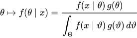
${\displaystyle \theta \mapsto f(\theta \mid x)={\frac {f(x\mid \theta )\,g(\theta )}{\displaystyle \int _{\Theta }f(x\mid \vartheta )\,g(\vartheta )\,d\vartheta }}\!}$

どこ${\displaystyle g}$は密度関数である${\displaystyle \theta }$、${\displaystyle \Theta }$は、${\displaystyle g}$。

最大事後確率推定法では、${\displaystyle \theta }$この確率変数の事後密度の最頻値として：

${\displaystyle {\begin{aligned}{\hat {\theta }}_{\mathrm {MAP} }(x)&={\underset {\theta }{\operatorname {arg\,max} }}\ f(\theta \mid x)\\&={\underset {\theta }{\operatorname {arg\,max} }}\ {\frac {f(x\mid \theta )\,g(\theta )}{\displaystyle \int _{\Theta }f(x\mid \vartheta )\,g(\vartheta )\,d\vartheta }}\\&={\underset {\theta }{\operatorname {arg\,max} }}\ f(x\mid \theta )\,g(\theta ).\end{aligned}}\!}$

事後密度（モデルの周辺尤度）の分母は常に正であり、${\displaystyle \theta }$したがって、最適化には関与しません。MAP推定値は${\displaystyle \theta }$事前分布が最尤推定値と一致する場合${\displaystyle g}$均一である（つまり、${\displaystyle g}$は定数関数であり、これは関数空間アプリケーションでよく見られるように、事前分布が参照尺度として採用されるときに発生します。

ベイズ推定量の文脈では、MAPはリスク関数を持つベイズリスクの最小化として復元できる。

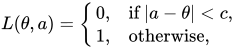
${\displaystyle L(\theta ,a)={\begin{cases}0,&{\text{if }}|a-\theta |<c,\\1,&{\text{otherwise}},\\\end{cases}}}$

極限では${\displaystyle c}$分布が 0 になる場合${\displaystyle \theta }$準凹関数である。^{[ 1 ]}ただし、一般的に、MAP推定量は、以下の条件を満たさない限り、ベイズ推定量ではない。${\displaystyle \theta }$離散的である。

MAP推定値は、いくつかの方法で計算できます。

1. 解析的に、事後確率密度の最頻値を閉じた形で与えることができる場合。これは共役事前分布を使用する場合に当てはまります。
2. 共役勾配法やニュートン法などの数値最適化法を用いる。通常、これには1階または2階導関数が必要となり、それらを解析的または数値的に評価する必要がある。
3. 期待値最大化アルゴリズムの改良版を用いる。この方法では事後確率密度関数の導関数は不要である。
4. シミュレーテッドアニーリングを用いたモンテカルロ法

MAP推定がベイズ推定の極限ケースとなるには、(0-1損失関数の下で) 緩やかな条件しか必要とされないが、^{[ 1 ]}ベイズ法全般を代表するものではない。これは、MAP推定が点推定であり、参照尺度の任意の選択に依存するのに対し、ベイズ法は分布を使用してデータを要約し、推論を行うことを特徴としているためである。したがって、ベイズ法は信頼区間とともに事後平均または中央値を報告する傾向がある。これは、これらの推定量がそれぞれ二乗誤差損失と線形誤差損失の下で最適であること（これらは典型的な損失関数をより代表している）と、連続的な事後分布に対してMAPが最適な点推定量であることを示唆する損失関数が存在しないという両方の理由による。

混合モデルなど、多くの種類のモデルでは、事後分布が多峰性になることがあります。このような場合、通常は最も高いモードを選択することが推奨されますが、これは常に可能とは限りません（グローバル最適化は難しい問題です）。また、識別可能性の問題が発生する場合など、場合によっては不可能なこともあります。さらに、特に多次元の場合、最も高いモードは事後分布の大部分の特徴を反映していない可能性があります。

最後に、ML推定器とは異なり、MAP推定値は再パラメータ化に対して不変ではありません。あるパラメータ化から別のパラメータ化に切り替えるには、最大値の位置に影響を与えるヤコビアンを導入する必要があります。 ^{[ 2 ]}対照的に、ベイズ事後期待値は再パラメータ化に対して不変です。

前述のベイズ推定器（平均推定器と中央値推定器）とMAP推定器の使用との違いの例として、入力を分類する必要がある場合を考えてみましょう。${\displaystyle x}$肯定的か否定的か（例えば、ローンをリスクが高いか安全か）に分類する。正しい分類方法について考えられる仮説が3つしかないと仮定する。${\displaystyle h_{1}}$、${\displaystyle h_{2}}$そして${\displaystyle h_{3}}$事後確率はそれぞれ0.4、0.3、0.3である。新しいインスタンスが与えられたと仮定すると、${\displaystyle x}$、${\displaystyle h_{1}}$1つは陽性と分類するが、他の2つは陰性と分類する。正しい分類器のMAP推定値を使用する${\displaystyle h_{1}}$、${\displaystyle x}$は陽性と分類されるが、ベイズ推定器はすべての仮説を平均して分類する。${\displaystyle x}$否定的な意味で。

数列が与えられたと仮定します${\displaystyle (x_{1},\dots ,x_{n})}$IIDの${\displaystyle N(\mu ,\sigma _{v}^{2})}$確率変数と事前分布${\displaystyle \mu }$は ${\displaystyle N(\mu _{0},\sigma _{m}^{2})}$MAP推定値を求めたい${\displaystyle \mu }$正規分布は自身の共役事前分布であるため、解析的に閉形式解を求めることができることに注意してください。

最大化すべき関数は^{[ 3 ]で与えられる。}

${\displaystyle g(\mu )f(x\mid \mu )=\pi (\mu )L(\mu )={\frac {1}{{\sqrt {2\pi }}\sigma _{m}}}\exp \left(-{\frac {1}{2}}\left({\frac {\mu -\mu _{0}}{\sigma _{m}}}\right)^{2}\right)\prod _{j=1}^{n}{\frac {1}{{\sqrt {2\pi }}\sigma _{v}}}\exp \left(-{\frac {1}{2}}\left({\frac {x_{j}-\mu }{\sigma _{v}}}\right)^{2}\right),}$

これは、次の関数を最小化することと同等です。${\displaystyle \mu }$:

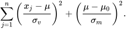
$\displaystyle \sum _{j=1}^{n}\left({\frac {x_{j}-\mu }{\sigma _{v}}}\right)^{2}+\left({\frac {\mu -\mu _{0}}{\sigma _{m}}}\right)^{2}.}$

したがって、 μのMAP推定量は^{[ 3 ]}で与えられることがわかります。

${\displaystyle {\hat {\mu }}_{\mathrm {MAP} }={\frac {\sigma _{m}^{2}\,n}{\sigma _{m}^{2}\,n+\sigma _{v}^{2}}}\left({\frac {1}{n}}\sum _{j=1}^{n}x_{j}\right)+{\frac {\sigma _{v}^{2}}{\sigma _{m}^{2}\,n+\sigma _{v}^{2}}}\,\mu _{0}={\frac {\sigma _{m}^{2}\left(\sum _{j=1}^{n}x_{j}\right)+\sigma _{v}^{2}\,\mu _{0}}{\sigma _{m}^{2}\,n+\sigma _{v}^{2}}}.}$

これは、事前平均と標本平均をそれぞれの共分散で重み付けした線形補間であることが判明した。

のケース$\displaystyle \sigma _{m}\to \infty }$これは非情報的な事前分布と呼ばれ、不適切な確率分布につながります。この場合${\displaystyle {\hat {\mu }}_{\mathrm {MAP} }\to {\hat {\mu }}_{\mathrm {MLE} }.}$

• デグルート、M. (1970).最適な統計的意思決定. マグロウヒル. ISBN 0-07-016242-5。
• ソレンソン、ハロルド・W. (1980).パラメータ推定：原理と問題. マルセル・デッカー. ISBN 0-8247-6987-2。
• Hald, Anders (2007). 「ガウスによる正規分布の導出と最小二乗法、1809年」。『ベルヌーイからフィッシャーまでのパラメトリック統計推論の歴史、1713年～1935年』。ニューヨーク：Springer。pp. 55–61。ISBN  978-0-387-46409-1。