内部根号を含む数式
代数学 において 、 ネストされた根号 とは、 根号式 (平方根記号、立方根記号などを含むもの)が別の根号式を含む(ネストする)ものである。例としては、
5 − 2
5
、
{\displaystyle {\sqrt {5-2{\sqrt {5}}\ }},}
これは正五角形 や、より複雑なものについて
議論するときに生じる。
2 +
3
+
4
3
3
。
{\displaystyle {\sqrt[{3}]{2+{\sqrt {3}}+{\sqrt[{3}]{4}}\ }}.}
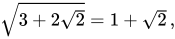
デネスティング ネストされた根号は、ネストされていない形式に書き直すことができます。たとえば、
3 + 2
2
= 1 +
2
、
{\displaystyle {\sqrt {3+2{\sqrt {2}}}}=1+{\sqrt {2}}\,,}
2
+
5 − 2
6
=
3
、
{\displaystyle {\sqrt {2}}+{\sqrt {5-2{\sqrt {6}}}}={\sqrt {3}},\quad }
[1]
2
3
− 1
3
=
1 −
2
3
+
4
3
9
3
。
{\displaystyle {\sqrt[{3}]{{\sqrt[{3}]{2}}-1}}={\frac {1-{\sqrt[{3}]{2}}+{\sqrt[{3}]{4}}}{\sqrt[{3}]{9}}}\,.}
もう一つの簡単な例を挙げると、
2
3
=
2
6
{\displaystyle {\sqrt[{3}]{\sqrt {2}}}={\sqrt[{6}]{2}}}
このようにネストされた根号を書き換えることを デネスティング と呼びます。これは常に可能であるとは限らず、可能であっても難しい場合がよくあります。
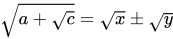
2つのネストされた平方根 2つの入れ子になった平方根の場合、次の定理は入れ子解除の問題を完全に解決します。 [2]
a と c が 有理数 であり 、 c が 有理数の平方でない 場合、 が有理数 d の平方である
場合に限り、 となる 2
つの有理数 x と y が存在します。
1つの +
c
=
x
±
ええ
{\displaystyle {\sqrt {a+{\sqrt {c}}}}={\sqrt {x}}\pm {\sqrt {y}}}
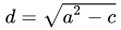
1つの
2
− c
{\displaystyle a^{2}-c~}
ネストされた根号が実数の場合、 x と y は 2 つの数値であり
、 は 有理数です。
1つの + d
2
{\displaystyle {\frac {a+d}{2}}~}
1つの − d
2
、
{\displaystyle ~{\frac {ad}{2}}~,~}
d =
1つの
2
− c
{\displaystyle ~d={\sqrt {a^{2}-c}}~}
特に、 a と c が 整数の場合、 2 x と 2 y は整数です。
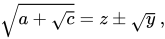
この結果には、 z は 常に記述でき 、項の少なくとも 1 つは正でなければならない (式の左辺が正であるため) という
形式 のネスト解除が含まれます
。
1つの +
c
= ず ±
ええ
、
{\displaystyle {\sqrt {a+{\sqrt {c}}}}=z\pm {\sqrt {y}}~,}
ず = ±
ず
2
、
{\displaystyle z=\pm {\sqrt {z^{2}}},}
より一般的なデネスティング式は、次 の形式になります。
ただし、 ガロア理論 では、左辺が に属するか 、または のいずれかまたは両方の符号を変更することによって取得する必要があることが示されています。最初のケースでは、これは x = c と取ることができることを意味します。2 番目のケース では、 もう 1 つの係数は 0 でなければなりません 。xy を x と名前 変更して を 取得すると、 同様に 進めると、 と仮定できます。 これは、明らかにより一般的なデネスティングが常に上記の 1 つに簡略化できることを示しています。
1つの +
c
= α + β
x
+ γ
ええ
+ δ
x
ええ
。
{\displaystyle {\sqrt {a+{\sqrt {c}}}}=\alpha +\beta {\sqrt {x}}+\gamma {\sqrt {y}}+\delta {\sqrt {x}}{\sqrt {y}}~.}
質問
(
c
) 、
{\displaystyle \mathbb {Q} ({\sqrt {c}}),}
x
、
{\displaystyle {\sqrt {x}},}
ええ
、
{\displaystyle {\sqrt {y}},}
γ = δ = 0.
{\displaystyle \gamma =\delta =0.}
α
{\displaystyle \alpha}
β = 0 、
{\displaystyle \beta =0,}
δ = 0.
{\displaystyle \delta =0.}
α = 0 、
{\displaystyle \alpha =0,}
α = δ = 0.
{\displaystyle \alpha =\delta =0.}
証明 :二乗すると、この式は
右辺がマイナスの場合は
、
1つの +
c
=
x
±
ええ
{\displaystyle {\sqrt {a+{\sqrt {c}}}}={\sqrt {x}}\pm {\sqrt {y}}}
1つの +
c
= x + ええ ± 2
x ええ
、
{\displaystyle a+{\sqrt {c}}=x+y\pm 2{\sqrt {xy}},}
| x | ≥ | y | 、
(平方根は記法の定義により非負である)。不等式は x と yを 入れ替えることで常に満たされる可能性があるため、最初の方程式を x と y で
解くことは、
1つの +
c
= x + ええ ± 2
x ええ
。
{\displaystyle a+{\sqrt {c}}=x+y\pm 2{\sqrt {xy}}.}
この等式は、が 二次方程式体 に属することを意味します。 この体では、すべての要素は 、およびが 有理数 であるとして一意に表すことができます。これは、が有理数ではないことを意味します( そう
でなければ、方程式の右辺は有理数になりますが、左辺は無理数になります)。 x と y は 有理数でなければならないので、 の平方は 有理数でなければなりません。これは、 の式において、 が であることを意味します。したがって
、ある有理数に対して 1
および 上の分解の一意性は 、 したがって、検討中の方程式が と同等であることを意味します
。 Vieta の公式 により、 x と y は 二次方程式 の根でなければならないこと
がわかります
( ≠ 0 、そうでなければ c は a の平方になります )。したがって、 x と y は であり
、
したがって、 が有理数である
場合に限り、 x と y は有理数です。
x ええ
{\displaystyle {\sqrt {xy}}}
質問
(
c
) 。
{\displaystyle \mathbb {Q} ({\sqrt {c}}).}
α + β
c
、
{\displaystyle \alpha +\beta {\sqrt {c}},}
α
{\displaystyle \alpha}
β
{\displaystyle \beta}
± 2
x ええ
{\displaystyle \pm 2{\sqrt {xy}}}
± 2
x ええ
{\displaystyle \pm 2{\sqrt {xy}}}
α = 0
{\displaystyle \alpha =0}
± 2
x ええ
{\displaystyle \pm 2{\sqrt {xy}}}
α + β
c
。
{\displaystyle \alpha +\beta {\sqrt {c}}.}
1つの +
c
= x + ええ + β
c
{\displaystyle a+{\sqrt {c}}=x+y+\beta {\sqrt {c}}}
β 。
{\displaystyle \beta .}
c
{\displaystyle {\sqrt {c}}}
1つの = x + ええ
そして
± 2
x ええ
=
c
。
{\displaystyle a=x+y\quad {\text{and}}\quad \pm 2{\sqrt {xy}}={\sqrt {c}}.}
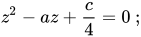
ず
2
− 1つの ず +
c 4
= 0
;
{\displaystyle z^{2}-az+{\frac {c}{4}}=0~;}
Δ =
1つの
2
− c =
d
2
> 0
{\displaystyle ~\Delta =a^{2}-c=d^{2}>0~}
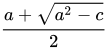
1つの +
1つの
2
− c
2
{\displaystyle {\frac {a+{\sqrt {a^{2}-c}}}{2}}~}
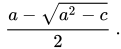
1つの −
1つの
2
− c
2
。
{\displaystyle ~{\frac {a-{\sqrt {a^{2}-c}}}{2}}~.}
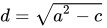
d =
1つの
2
− c
{\displaystyle d={\sqrt {a^{2}-c}}~}
さまざまな符号を明示的に選択するには、正の実数の平方根のみを考慮する必要があり、したがって c > 0 と仮定します。この式は、 | a | > √ c であることを示しています 。したがって、ネストされた根号が実数で、ネスト解除が可能な場合は、 a > 0 です。すると、解は次のようになります。
1つの
2
= c +
d
2
{\displaystyle a^{2}=c+d^{2}}
1つの +
c
=
1つの + d
2
+
1つの − d
2
、
1つの −
c
=
1つの + d
2
−
1つの − d
2
。
{\displaystyle {\begin{aligned}{\sqrt {a+{\sqrt {c}}}}&={\sqrt {\frac {a+d}{2}}}+{\sqrt {\frac {ad}{2}}},\\[6pt]{\sqrt {a-{\sqrt {c}}}}&={\sqrt {\frac {a+d}{2}}}-{\sqrt {\frac {ad}{2}}}.\end{aligned}}}
ラマヌジャンのいくつかのアイデンティティ シュリニヴァーサ・ラマヌジャンは、 入れ子になった根号を含むいくつかの興味深い恒等式を示した。その中には次のようなものがある: [3]
3 + 2
5
4
3 − 2
5
4
4
=
5
4
+ 1
5
4
− 1
=
1 2
(
3 +
5
4
+
5
+
125
4
)
、
{\displaystyle {\sqrt[{4}]{\frac {3+2{\sqrt[{4}]{5}}}{3-2{\sqrt[{4}]{5}}}}}={\frac {{\sqrt[{4}]{5}}+1}{{\sqrt[{4}]{5}}-1}}={\tfrac {1}{2}}\left(3+{\sqrt[{4}]{5}}+{\sqrt {5}}+{\sqrt[{4}]{125}}\right),}
28
3
−
27
3
=
1 3
(
98
3
−
28
3
− 1
)
、
{\displaystyle {\sqrt {{\sqrt[{3}]{28}}-{\sqrt[{3}]{27}}}}={\tfrac {1}{3}}\left({\sqrt[{3}]{98}}-{\sqrt[{3}]{28}}-1\right),}
32 5
5
−
27 5
5
3
=
1 25
5
+
3 25
5
−
9 25
5
、
{\displaystyle {\sqrt[{3}]{{\sqrt[{5}]{\frac {32}{5}}}-{\sqrt[{5}]{\frac {27}{5}}}}}={\sqrt[{5}]{\frac {1}{25}}}+{\sqrt[{5}]{\frac {3}{25}}}-{\sqrt[{5}]{\frac {9}{25}}},}
そして
2
3
− 1
3
=
1 9
3
−
2 9
3
+
4 9
3
。
{\displaystyle {\sqrt[{3}]{\ {\sqrt[{3}]{2}}\ -1}}={\sqrt[{3}]{\frac {1}{9}}}-{\sqrt[{3}]{\frac {2}{9}}}+{\sqrt[{3}]{\frac {4}{9}}}.\quad }
[4]
ランダウのアルゴリズム 1989年、 スーザン・ランドーは、 どのネストされた根号をデネストできるかを決定する 最初の アルゴリズムを発表しました。 [5] 以前のアルゴリズムは、いくつかのケースでは機能しましたが、他のケースでは機能しませんでした。ランドーのアルゴリズムは、 1の複素根 を扱い、ネストされた根号の深さに応じて 指数時間 で実行されます。 [6]
三角法では 三角法 では 、多くの角度の 正弦と余弦を 入れ子の根号で表すことができます。たとえば、
sin
π
60
=
sin
3
∘
=
1
16
[
2
(
1
−
3
)
5
+
5
+
2
(
5
−
1
)
(
3
+
1
)
]
{\displaystyle \sin {\frac {\pi }{60}}=\sin 3^{\circ }={\frac {1}{16}}\left[2(1-{\sqrt {3}}){\sqrt {5+{\sqrt {5}}}}+{\sqrt {2}}({\sqrt {5}}-1)({\sqrt {3}}+1)\right]}
最後の等式は、
§ 2 つのネストされた平方根の結果から直接生じます。
sin
π
24
=
sin
7.5
∘
=
1
2
2
−
2
+
3
=
1
2
2
−
1
+
3
2
.
{\displaystyle \sin {\frac {\pi }{24}}=\sin 7.5^{\circ }={\frac {1}{2}}{\sqrt {2-{\sqrt {2+{\sqrt {3}}}}}}={\frac {1}{2}}{\sqrt {2-{\frac {1+{\sqrt {3}}}{\sqrt {2}}}}}.}
三次方程式の解において 3次方程式 の 代数解 にはネストされた根号が現れる 。任意の3次方程式は、2次項を使わずに簡略化した形で次のように表すことができる。
x
3
+
p
x
+
q
=
0
,
{\displaystyle x^{3}+px+q=0,}
その根の1つに対する一般解は
x
=
−
q
2
+
q
2
4
+
p
3
27
3
+
−
q
2
−
q
2
4
+
p
3
27
3
.
{\displaystyle x={\sqrt[{3}]{-{q \over 2}+{\sqrt {{q^{2} \over 4}+{p^{3} \over 27}}}}}+{\sqrt[{3}]{-{q \over 2}-{\sqrt {{q^{2} \over 4}+{p^{3} \over 27}}}}}.}
3次方程式に実根が1つしかない場合、実根は、3次根の 被根号 が実数で、3次根が実数3次根であるこの式で与えられます。実根が3つある場合、平方根の式は虚数です。ここで、実根は、最初の3次根を複素被根号の任意の特定の複素3次根と定義し、2番目の3次根を最初の3次根の 複素共役 と定義することによって表されます。この解のネストされた根号は、3次方程式に少なくとも1つの 有 理解がない限り、一般に簡略化できません。実際、3次方程式に無理数ではあるが実数の解が3つある場合、 3つの実数解がすべて複素数の3次根で表された casus irreducibilis があります。一方、次の式を考えてみましょう。
x
3
−
7
x
+
6
=
0
,
{\displaystyle x^{3}-7x+6=0,}
有理解1、2、-3を持つ。上記の一般解の式は、解を与える。
x
=
−
3
+
10
3
i
9
3
+
−
3
−
10
3
i
9
3
.
{\displaystyle x={\sqrt[{3}]{-3+{\frac {10{\sqrt {3}}i}{9}}}}+{\sqrt[{3}]{-3-{\frac {10{\sqrt {3}}i}{9}}}}.}
立方根とその共役の任意の選択に対して、これには複素数を含むネストされた根号が含まれますが、(明らかではないにしても) 解 1、2、または -3 のいずれかに簡約できます。
無限にネストされた根号
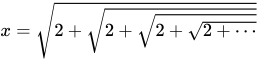
平方根 特定の条件下では、無限にネストされた平方根、例えば
x
=
2
+
2
+
2
+
2
+
⋯
{\displaystyle x={\sqrt {2+{\sqrt {2+{\sqrt {2+{\sqrt {2+\cdots }}}}}}}}}
は有理数を表します。この有理数は、 xが 根号の下にも現れる
ことに気づくことで見つけられ、次の式が得られます。
x
=
2
+
x
.
{\displaystyle x={\sqrt {2+x}}.}
この方程式を解くと、 x = 2 であることがわかります(2番目の解 x = −1 は、正の平方根を意味するという慣例の下では適用されません)。このアプローチは、一般に n > 0 の場合、
n
+
n
+
n
+
n
+
⋯
=
1
2
(
1
+
1
+
4
n
)
{\displaystyle {\sqrt {n+{\sqrt {n+{\sqrt {n+{\sqrt {n+\cdots }}}}}}}}={\tfrac {1}{2}}\left(1+{\sqrt {1+4n}}\right)}
は方程式 x 2 − x − n = 0 の正の根です。 n = 1 の場合、この根は 黄金比 φで、約 1.618 に等しくなります。 n > 0 の場合、
同じ手順で方程式 x 2 + x − n = 0
の正の根 も得られます 。
n
−
n
−
n
−
n
−
⋯
=
1
2
(
−
1
+
1
+
4
n
)
,
{\displaystyle {\sqrt {n-{\sqrt {n-{\sqrt {n-{\sqrt {n-\cdots }}}}}}}}={\tfrac {1}{2}}\left(-1+{\sqrt {1+4n}}\right),}
2 のネストされた平方根 2の入れ子になった平方根は、無限に入れ子になった根号の広いクラスの特別なケースです。これらを 正弦と余弦に結びつける結果は数多く知られています。たとえば、2の入れ子になった平方根は [7] のように表されます。
R
(
b
k
,
…
,
b
1
)
=
b
k
2
2
+
b
k
−
1
2
+
b
k
−
2
2
+
⋯
+
b
2
2
+
x
{\displaystyle R(b_{k},\ldots ,b_{1})={\frac {b_{k}}{2}}{\sqrt {2+b_{k-1}{\sqrt {2+b_{k-2}{\sqrt {2+\cdots +b_{2}{\sqrt {2+x}}}}}}}}}
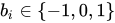
ここで、は [−2,2] の範囲内に あり、 に対しては 、 に対しては
x
=
2
sin
(
π
b
1
/
4
)
{\displaystyle x=2\sin(\pi b_{1}/4)}
b
1
{\displaystyle b_{1}}
b
i
∈
{
−
1
,
0
,
1
}
{\displaystyle b_{i}\in \{-1,0,1\}}
i
≠
1
{\displaystyle i\neq 1}
R
(
b
k
,
…
,
b
1
)
=
cos
θ
{\displaystyle R(b_{k},\ldots ,b_{1})=\cos \theta }
θ
=
(
1
2
−
b
k
4
−
b
k
b
k
−
1
8
−
b
k
b
k
−
1
b
k
−
2
16
−
⋯
−
b
k
b
k
−
1
⋯
b
1
2
k
+
1
)
π
.
{\displaystyle \theta =\left({\frac {1}{2}}-{\frac {b_{k}}{4}}-{\frac {b_{k}b_{k-1}}{8}}-{\frac {b_{k}b_{k-1}b_{k-2}}{16}}-\cdots -{\frac {b_{k}b_{k-1}\cdots b_{1}}{2^{k+1}}}\right)\pi .}
この結果から、 k個のネストされた根からなる次の無限ネストされた根号の任意の値
を次のように推定することができる。
x
∈
[
−
2
,
2
]
{\displaystyle x\in [-2,2]}
R
k
(
x
)
=
2
+
2
+
⋯
+
2
+
x
.
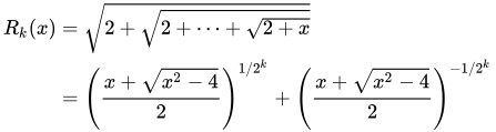
{\displaystyle R_{k}(x)={\sqrt {2+{\sqrt {2+\cdots +{\sqrt {2+x}}}}}}.}
もし 、ならば [8]
x
≥
2
{\displaystyle x\geq 2}
R
k
(
x
)
=
2
+
2
+
⋯
+
2
+
x
=
(
x
+
x
2
−
4
2
)
1
/
2
k
+
(
x
+
x
2
−
4
2
)
−
1
/
2
k
{\displaystyle {\begin{aligned}R_{k}(x)&={\sqrt {2+{\sqrt {2+\cdots +{\sqrt {2+x}}}}}}\\&=\left({\frac {x+{\sqrt {x^{2}-4}}}{2}}\right)^{1/2^{k}}+\left({\frac {x+{\sqrt {x^{2}-4}}}{2}}\right)^{-1/2^{k}}\end{aligned}}}
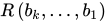
これらの結果は、の入れ子になった平方根表現を得るために使用できます 。上で定義した項を考えてみましょう 。すると [7]
π
{\displaystyle \pi }
R
(
b
k
,
…
,
b
1
)
{\displaystyle R\left(b_{k},\ldots ,b_{1}\right)}
π
=
lim
k
→
∞
[
2
k
+
1
2
−
b
1
R
(
1
,
−
1
,
1
,
1
,
…
,
1
,
1
,
b
1
⏟
k
terms
)
]
{\displaystyle \pi =\lim _{k\rightarrow \infty }\left[{\frac {2^{k+1}}{2-b_{1}}}R(\underbrace {1,-1,1,1,\ldots ,1,1,b_{1}} _{k{\text{ terms }}})\right]}
どこ 。
b
1
≠
2
{\displaystyle b_{1}\neq 2}
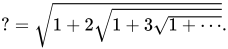
ラマヌジャンの無限根号 ラマヌジャンは インド数学会誌 に次のような問題を提起した 。
?
=
1
+
2
1
+
3
1
+
⋯
.
{\displaystyle ?={\sqrt {1+2{\sqrt {1+3{\sqrt {1+\cdots }}}}}}.}
これは、より一般的な定式化に注目することで解決できます。
?
=
a
x
+
(
n
+
a
)
2
+
x
a
(
x
+
n
)
+
(
n
+
a
)
2
+
(
x
+
n
)
⋯
.
{\displaystyle ?={\sqrt {ax+(n+a)^{2}+x{\sqrt {a(x+n)+(n+a)^{2}+(x+n){\sqrt {\mathrm {\cdots } }}}}}}.}
これをF ( x ) とし 、両辺を二乗すると次のようになる。
F
(
x
)
2
=
a
x
+
(
n
+
a
)
2
+
x
a
(
x
+
n
)
+
(
n
+
a
)
2
+
(
x
+
n
)
⋯
,
{\displaystyle F(x)^{2}=ax+(n+a)^{2}+x{\sqrt {a(x+n)+(n+a)^{2}+(x+n){\sqrt {\mathrm {\cdots } }}}},}
これを簡略化すると
F
(
x
)
2
=
a
x
+
(
n
+
a
)
2
+
x
F
(
x
+
n
)
.
{\displaystyle F(x)^{2}=ax+(n+a)^{2}+xF(x+n).}
それは次のことが証明できる
F
(
x
)
=
x
+
n
+
a
{\displaystyle F(x)={x+n+a}}
は の方程式を満たすので 、これが真の解であると期待できます。完全な証明のためには、これが実際に の方程式の解であることを示す必要があります 。
F
(
x
)
{\displaystyle F(x)}
F
(
x
)
{\displaystyle F(x)}
そこで、 a = 0 、 n = 1 、 x = 2 とすると、
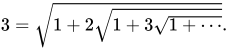
ラマヌジャンは 失われたノート
の中で、次のような無限根号のネスティングを述べている 。
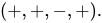
記号の繰り返しパターンは、
3
=
1
+
2
1
+
3
1
+
⋯
.
{\displaystyle 3={\sqrt {1+2{\sqrt {1+3{\sqrt {1+\cdots }}}}}}.}
5
+
5
+
5
−
5
+
5
+
5
+
5
−
⋯
=
2
+
5
+
15
−
6
5
2
.
{\displaystyle {\sqrt {5+{\sqrt {5+{\sqrt {5-{\sqrt {5+{\sqrt {5+{\sqrt {5+{\sqrt {5-\cdots }}}}}}}}}}}}}}={\frac {2+{\sqrt {5}}+{\sqrt {15-6{\sqrt {5}}}}}{2}}.}
(
+
,
+
,
−
,
+
)
.
{\displaystyle (+,+,-,+).}
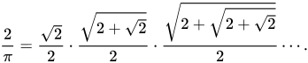
ヴィエトの表現 π 円周と直径の比
π の ビエトの公式は、
2
π
=
2
2
⋅
2
+
2
2
⋅
2
+
2
+
2
2
⋯
.
{\displaystyle {\frac {2}{\pi }}={\frac {\sqrt {2}}{2}}\cdot {\frac {\sqrt {2+{\sqrt {2}}}}{2}}\cdot {\frac {\sqrt {2+{\sqrt {2+{\sqrt {2}}}}}}{2}}\cdots .}
立方根 場合によっては、無限にネストされた立方根、例えば は
有理数も表すことができます。ここでも、式全体がそれ自身の中に現れることに気づくと、次の式が残ります。
x
=
6
+
6
+
6
+
6
+
⋯
3
3
3
3
{\displaystyle x={\sqrt[{3}]{6+{\sqrt[{3}]{6+{\sqrt[{3}]{6+{\sqrt[{3}]{6+\cdots }}}}}}}}}
x
=
6
+
x
3
.
{\displaystyle x={\sqrt[{3}]{6+x}}.}
この方程式を解くと、 x = 2 であることがわかります。より一般的には、 は
すべての n > 0に対して方程式 x 3 − x − n = 0
の正の実根であることがわかります 。 n = 1 の場合、この根は 塑性比 ρ で、およそ 1.3247 に等しくなります。
n
+
n
+
n
+
n
+
⋯
3
3
3
3
{\displaystyle {\sqrt[{3}]{n+{\sqrt[{3}]{n+{\sqrt[{3}]{n+{\sqrt[{3}]{n+\cdots }}}}}}}}}
同じ手順で
n
−
n
−
n
−
n
−
⋯
3
3
3
3
{\displaystyle {\sqrt[{3}]{n-{\sqrt[{3}]{n-{\sqrt[{3}]{n-{\sqrt[{3}]{n-\cdots }}}}}}}}}
すべてのn > 1 に対して 方程式 x 3 + x − n = 0 の実根として。
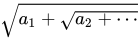
ハーシュフェルトの収束定理 無限にネストされた根号 (すべて 非負)が収束するの は 、 すべての に対して となるような ものが存在する場合のみである [9] 。言い換えれば、
a
1
+
a
2
+
⋯
{\displaystyle {\sqrt {a_{1}+{\sqrt {a_{2}+\dotsb }}}}}
a
i
{\displaystyle a_{i}}
M
∈
R
{\displaystyle M\in \mathbb {R} }
M
≥
a
n
2
−
n
{\displaystyle M\geq a_{n}^{2^{-n}}}
n
{\displaystyle n}
sup
a
n
2
−
n
<
+
∞
.
{\textstyle \sup a_{n}^{2^{-n}}<+\infty .}
「もし」の証明
さらに、この数列は単調増加である ことがわかります
。したがって、 単調収束定理 により、収束します。
a
1
+
a
2
+
⋯
≤
M
2
1
+
M
2
2
+
⋯
=
M
1
+
1
+
⋯
<
2
M
.
{\displaystyle {\sqrt {a_{1}+{\sqrt {a_{2}+\dotsb }}}}\leq {\sqrt {M^{2^{1}}+{\sqrt {M^{2^{2}}+\cdots }}}}=M{\sqrt {1+{\sqrt {1+\dotsb }}}}<2M.}
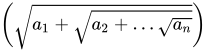
(
a
1
+
a
2
+
…
a
n
)
{\displaystyle \left({\sqrt {a_{1}+{\sqrt {a_{2}+\dotsc {\sqrt {a_{n}}}}}}}\right)}
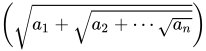
「もしあれば」の証明 シーケンスが 収束する場合、それは有界です。
(
a
1
+
a
2
+
⋯
a
n
)
{\displaystyle \left({\sqrt {a_{1}+{\sqrt {a_{2}+\cdots {\sqrt {a_{n}}}}}}}\right)}
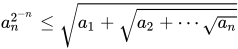
しかし、 なので も有界です。
a
n
2
−
n
≤
a
1
+
a
2
+
⋯
a
n
{\displaystyle a_{n}^{2^{-n}}\leq {\sqrt {a_{1}+{\sqrt {a_{2}+\cdots {\sqrt {a_{n}}}}}}}}
(
a
n
2
−
n
)
{\displaystyle \left(a_{n}^{2^{-n}}\right)}
参照
参考文献
^ シェイナーマン、エドワード R. (2000)、「十分に近いときは十分に近い」、 アメリカ数学月刊誌 、 107 (6): 489–499、 doi :10.2307/2589344、 JSTOR 2589344、 MR 1766736 ^ オイラー、レオンハルト (2012). 代数の要素 . Springer Science & Business Media. 第8章. ^ Landau, Susan (1993年7月16日). 「「Zippel Denesting」に関する注記」. CiteSeerX 10.1.1.35.5512 . 2023年 8月23日 閲覧 。 ^ Berndt, Bruce; Chan, Heng; Zhang, Liang-Cheng (1998). 「ラマヌジャンの著作における根号と単位」 (PDF) . Acta Arithmetica . 87 (2): 145–158. doi : 10.4064/aa-87-2-145-158 . ^ Landau, Susan (1992). 「ネストされたラジカルの簡略化」. 30th Annual Symposium on Foundations of Computer Science . Vol. 21. SIAM . pp. 85–110. CiteSeerX 10.1.1.34.2003 . doi :10.1109/SFCS.1989.63496. ISBN 978-0-8186-1982-3 . S2CID 29982884。 ^ Gkioulekas, Eleftherios (2017-08-18). 「ネストされた平方根のデネスティングについて」. 国際科学技術数学教育ジャーナル . 48 (6): 942–953. Bibcode :2017IJMES..48..942G. doi :10.1080/0020739X.2017.1290831. ISSN 0020-739X. S2CID 9737528. ^ ab Servi, LD (2003年4月). 「2のネストされた平方根」. アメリカ数学月刊誌 . 110 (4): 326–330. doi :10.1080/00029890.2003.11919968. ISSN 0002-9890. S2CID 38100940. ^ Nyblom, MA (2005 年 11 月). 「More Nested Square Roots of 2」. The American Mathematical Monthly . 112 (9): 822–825. doi :10.1080/00029890.2005.11920256. ISSN 0002-9890. S2CID 11206345. ^ Herschfeld, Aaron (1935). 「無限根号について」. アメリカ数学月刊誌 . 42 (7): 419–429. doi :10.2307/2301294. ISSN 0002-9890. JSTOR 2301294.
さらに読む 

![{\displaystyle {\sqrt[{3}]{2+{\sqrt {3}}+{\sqrt[{3}]{4}}\ }}.}](https://wikimedia.org/api/rest_v1/media/math/render/svg/16622bdbf373e2237bfac23a3c7cf619353e851e)

![{\displaystyle {\sqrt[{3}]{{\sqrt[{3}]{2}}-1}}={\frac {1-{\sqrt[{3}]{2}}+{\sqrt[{3}]{4}}}{\sqrt[{3}]{9}}}\,.}](https://wikimedia.org/api/rest_v1/media/math/render/svg/a9a0cacad52ba247ccc394608bc1d35f054ca453)
![{\displaystyle {\sqrt[{3}]{\sqrt {2}}}={\sqrt[{6}]{2}}}](https://wikimedia.org/api/rest_v1/media/math/render/svg/8db3a5d203b3b6a4cf20423ca70cd1238cca922b)
















![{\displaystyle {\begin{aligned}{\sqrt {a+{\sqrt {c}}}}&={\sqrt {\frac {a+d}{2}}}+{\sqrt {\frac {ad}{2}}},\\[6pt]{\sqrt {a-{\sqrt {c}}}}&={\sqrt {\frac {a+d}{2}}}-{\sqrt {\frac {ad}{2}}}.\end{aligned}}}](https://wikimedia.org/api/rest_v1/media/math/render/svg/0286035e658c68e28f1d240f415b88d23e629eff)
![{\displaystyle {\sqrt[{4}]{\frac {3+2{\sqrt[{4}]{5}}}{3-2{\sqrt[{4}]{5}}}}}={\frac {{\sqrt[{4}]{5}}+1}{{\sqrt[{4}]{5}}-1}}={\tfrac {1}{2}}\left(3+{\sqrt[{4}]{5}}+{\sqrt {5}}+{\sqrt[{4}]{125}}\right),}](https://wikimedia.org/api/rest_v1/media/math/render/svg/027f261d646f8a48895ad0b0153bfc6748cb93dc)
![{\displaystyle {\sqrt {{\sqrt[{3}]{28}}-{\sqrt[{3}]{27}}}}={\tfrac {1}{3}}\left({\sqrt[{3}]{98}}-{\sqrt[{3}]{28}}-1\right),}](https://wikimedia.org/api/rest_v1/media/math/render/svg/3444106b707ba14d569e2cf1de20d8dbc40e5448)
![{\displaystyle {\sqrt[{3}]{{\sqrt[{5}]{\frac {32}{5}}}-{\sqrt[{5}]{\frac {27}{5}}}}}={\sqrt[{5}]{\frac {1}{25}}}+{\sqrt[{5}]{\frac {3}{25}}}-{\sqrt[{5}]{\frac {9}{25}}},}](https://wikimedia.org/api/rest_v1/media/math/render/svg/f58849bde3247783bf5d785a1e9559aaab78b6b6)
![{\displaystyle {\sqrt[{3}]{\ {\sqrt[{3}]{2}}\ -1}}={\sqrt[{3}]{\frac {1}{9}}}-{\sqrt[{3}]{\frac {2}{9}}}+{\sqrt[{3}]{\frac {4}{9}}}.\quad }](https://wikimedia.org/api/rest_v1/media/math/render/svg/b3c9504523719b9715ac6d1b7f0019890c2a4ff2)
![{\displaystyle \sin {\frac {\pi }{60}}=\sin 3^{\circ }={\frac {1}{16}}\left[2(1-{\sqrt {3}}){\sqrt {5+{\sqrt {5}}}}+{\sqrt {2}}({\sqrt {5}}-1)({\sqrt {3}}+1)\right]}](https://wikimedia.org/api/rest_v1/media/math/render/svg/826adb0a6f4d6fa33d4b638e89152b47c3e1941e)


![{\displaystyle x={\sqrt[{3}]{-{q \over 2}+{\sqrt {{q^{2} \over 4}+{p^{3} \over 27}}}}}+{\sqrt[{3}]{-{q \over 2}-{\sqrt {{q^{2} \over 4}+{p^{3} \over 27}}}}}.}}](https://wikimedia.org/api/rest_v1/media/math/render/svg/db7782b96c3abed7e27961869314809ae100b043)

![{\displaystyle x={\sqrt[{3}]{-3+{\frac {10{\sqrt {3}}i}{9}}}}+{\sqrt[{3}]{-3-{\frac {10{\sqrt {3}}i}{9}}}}.}](https://wikimedia.org/api/rest_v1/media/math/render/svg/1a2318662ab0606d8e4b345d27cc0ccdcacdb409)









![{\displaystyle x\in [-2,2]}](https://wikimedia.org/api/rest_v1/media/math/render/svg/21ba460b866dca981758622699215cc9bd96a3c5)



![{\displaystyle \pi =\lim _{k\rightarrow \infty }\left[{\frac {2^{k+1}}{2-b_{1}}}R(\underbrace {1,-1,1,1,\ldots ,1,1,b_{1}} _{k{\text{ 項 }}})\right]}](https://wikimedia.org/api/rest_v1/media/math/render/svg/3cef83b87ab02f3f6d9cea1040f79a74610e598c)







![{\displaystyle x={\sqrt[{3}]{6+{\sqrt[{3}]{6+{\sqrt[{3}]{6+{\sqrt[{3}]{6+\cdots }}}}}}}}}](https://wikimedia.org/api/rest_v1/media/math/render/svg/ec7ffe929585e38027f9ba3637b541f6157015b1)
![{\displaystyle x={\sqrt[{3}]{6+x}}.}](https://wikimedia.org/api/rest_v1/media/math/render/svg/b7629a30f94bd3edc8dc072f7820e325927fe3a2)
![{\displaystyle {\sqrt[{3}]{n+{\sqrt[{3}]{n+{\sqrt[{3}]{n+{\sqrt[{3}]{n+\cdots }}}}}}}}}](https://wikimedia.org/api/rest_v1/media/math/render/svg/a80cd88ecac26866718b70e587a4eb5207fa1dbb)
![{\displaystyle {\sqrt[{3}]{n-{\sqrt[{3}]{n-{\sqrt[{3}]{n-{\sqrt[{3}]{n-\cdots }}}}}}}}}](https://wikimedia.org/api/rest_v1/media/math/render/svg/e71a7a2dc6f241774cbc4c67d3784ed1fbbdd957)