意味
連続シャーレットシステム 複数のパラメータ a および s を用いた放物線状のスケーリングとせん断の幾何学的効果。
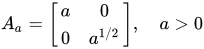
連続シャーレットシステムの構築は、放物線状のスケーリング行列に基づいている。
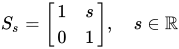
A 1 = [ 1 0 0 1 1 / 2 ] 、 1 > 0 {\displaystyle A_{a}={\begin{bmatrix}a&0\\0&a^{1/2}\end{bmatrix}},\quad a>0} 解像度を変更する手段として、せん断マトリックス上で
S s = [ 1 s 0 1 ] 、 s ∈ R {\displaystyle S_{s}={\begin{bmatrix}1&s\\0&1\end{bmatrix}},\quad s\in \mathbb {R} } 方向を変更する手段として、そして最後に位置を変更するために平行移動を使用します。カーブレット と比較すると、シアレットは回転の代わりにせん断を使用します。利点は、せん断演算子がS s {\displaystyle S_{s}} 整数格子 は、s ∈ Z {\displaystyle s\in \mathbb {Z} } S s Z 2 ⊆ Z 2 。 {\displaystyle S_{s}\mathbb {Z} ^{2}\subseteq \mathbb {Z} ^{2}.}
のためにψ ∈ L 2 ( R 2 ) \displaystyle \psi \in L^{2}(\mathbb {R} ^{2})} シャーレットシステム によって生成されるψ {\displaystyle \psi }
SH c o n t ( ψ ) = { ψ 1 、 s 、 t = 1 3 / 4 ψ ( S s A 1 ( ⋅ − t ) ) ∣ 1 > 0 、 s ∈ R 、 t ∈ R 2 } 、 {\displaystyle \operatorname {SH} _{\mathrm {cont} }(\psi )=\{\psi _{a,s,t}=a^{3/4}\psi (S_{s}A_{a}(\cdot -t))\mid a>0,s\in \mathbb {R} ,t\in \mathbb {R} ^{2}\},} 対応する連続シャーレット変換は 、次の写像で与えられる。
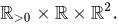
f ↦ S H ψ f ( 1 、 s 、 t ) = ⟨ f 、 ψ 1 、 s 、 t ⟩ 、 f ∈ L 2 ( R 2 ) 、 ( 1 、 s 、 t ) ∈ R > 0 × R × R 2 。 {\displaystyle f\mapsto {\mathcal {SH}}_{\psi }f(a,s,t)=\langle f,\psi _{a,s,t}\rangle ,\quad f\in L^{2}(\mathbb {R} ^{2}),\quad (a,s,t)\in \mathbb {R} _{>0}\times \mathbb {R} \times \mathbb {R} ^{2}.}
離散シャーレットシステム シャーレットシステムの離散バージョンは、以下から直接取得できます。SH c o n t ( ψ ) {\displaystyle \operatorname {SH} _{\mathrm {cont} }(\psi )} を離散化する ことによってR > 0 × R × R 2 。 \displaystyle \mathbb {R} _{>0}\times \mathbb {R} \times \mathbb {R} ^{2}.}
{ ( 2 j 、 k 、 A 2 j − 1 S k − 1 m ) ∣ j ∈ Z 、 k ∈ Z 、 m ∈ Z 2 } ⊆ R > 0 × R × R 2 。 {\displaystyle \{(2^{j},k,A_{2^{j}}^{-1}S_{k}^{-1}m)\mid j\in \mathbb {Z} ,k\in \mathbb {Z} ,m\in \mathbb {Z} ^{2}\}\subseteq \mathbb {R} _{>0}\times \mathbb {R} \times \mathbb {R} ^{2}.} このことから、シャーレット発生器に関連付けられた離散シャーレットシステムが得られる。 ψ {\displaystyle \psi }
SH ( ψ ) = { ψ j 、 k 、 m = 2 3 j / 4 ψ ( S k A 2 j ⋅ − m ) ∣ j ∈ Z 、 k ∈ Z 、 m ∈ Z 2 } 、 {\displaystyle \operatorname {SH} (\psi )=\{\psi _{j,k,m}=2^{3j/4}\psi (S_{k}A_{2^{j}}\cdot {}-m)\mid j\in \mathbb {Z} ,k\in \mathbb {Z} ,m\in \mathbb {Z} ^{2}\},} また、関連する離散シャーレット変換は 次のように定義される。
f ↦ S H ψ f ( j 、 k 、 m ) = ⟨ f 、 ψ j 、 k 、 m ⟩ 、 f ∈ L 2 ( R 2 ) 、 ( j 、 k 、 m ) ∈ Z × Z × Z 2 。 \displaystyle f\mapsto {\mathcal {SH}}_{\psi }f(j,k,m)=\langle f,\psi _{j,k,m}\rangle ,\quad f\in L^{2}(\mathbb {R} ^{2}),\quad (j,k,m)\in \mathbb {Z} \times \mathbb {Z} \times \mathbb {Z} ^{2}.}
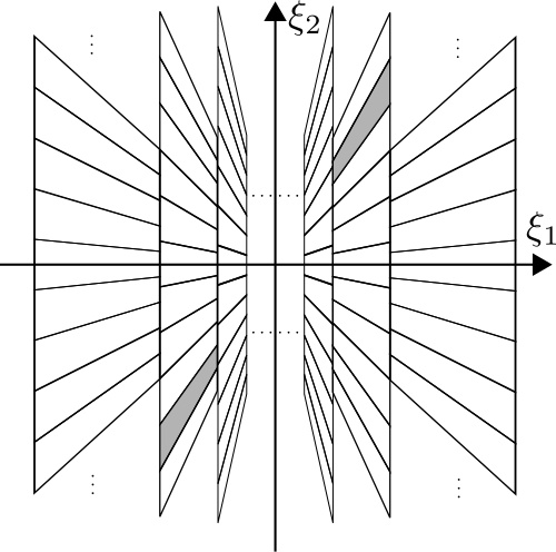
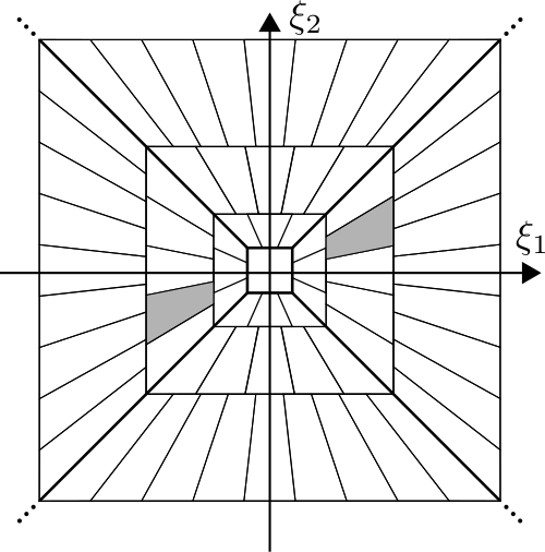
例 (離散的な)古典的なシャーレットシステムの周波数タイリング。
させてψ 1 ∈ L 2 ( R ) {\displaystyle \psi _{1}\in L^{2}(\mathbb {R} )} 離散カルデロン条件を満たす 関数、すなわち、
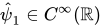
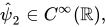
∑ j ∈ Z | ψ ^ 1 ( 2 − j ξ ) | 2 = 1 、 ae の場合 ξ ∈ R 、 {\displaystyle \sum _{j\in \mathbb {Z} }|{\hat {\psi }}_{1}(2^{-j}\xi )|^{2}=1,{\text{for ae }}\xi \in \mathbb {R} ,} とψ ^ 1 ∈ C ∞ ( R ) \displaystyle {\hat {\psi }}_{1}\in C^{\infty }(\mathbb {R} )} 補足 ψ ^ 1 ⊆ [ − 1 2 、 − 1 16 ] ∪ [ 1 16 、 1 2 ] 、 {\displaystyle \operatorname {supp} {\hat {\psi }}_{1}\subseteq [-{\tfrac {1}{2}},-{\tfrac {1}{16}}]\cup [{\tfrac {1}{16}},{\tfrac {1}{2}}],} ψ ^ 1 {\displaystyle {\hat {\psi }}_{1}} はフーリエ変換 を表す。ψ 1 。 {\displaystyle \psi _{1}.} ψ 1 {\displaystyle \psi _{1}} マイヤーウェーブレット である。さらに、ψ 2 ∈ L 2 ( R ) {\displaystyle \psi _{2}\in L^{2}(\mathbb {R} )} ψ ^ 2 ∈ C ∞ ( R ) 、 {\displaystyle {\hat {\psi }}_{2}\in C^{\infty }(\mathbb {R} ),} 補足 ψ ^ 2 ⊆ [ − 1 、 1 ] {\displaystyle \operatorname {supp} {\hat {\psi }}_{2}\subseteq [-1,1]}
∑ k = − 1 1 | ψ ^ 2 ( ξ + k ) | 2 = 1 、 ae の場合 ξ ∈ [ − 1 、 1 ] 。 {\displaystyle \sum _{k=-1}^{1}|{\hat {\psi }}_{2}(\xi +k)|^{2}=1,{\text{for a.e. }}\xi \in \left[-1,1\right].} 一般的には、ψ ^ 2 {\displaystyle {\hat {\psi }}_{2}} 滑らかな凹凸関数 となる。ψ ∈ L 2 ( R 2 ) {\displaystyle \psi \in L^{2}(\mathbb {R} ^{2})}
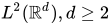
ψ ^ ( ξ ) = ψ ^ 1 ( ξ 1 ) ψ ^ 2 ( ξ 2 ξ 1 ) 、 ξ = ( ξ 1 、 ξ 2 ) ∈ R 2 、 {\displaystyle {\hat {\psi }}(\xi )={\hat {\psi }}_{1}(\xi _{1}){\hat {\psi }}_{2}\left({\tfrac {\xi _{2}}{\xi _{1}}}\right),\quad \xi =(\xi _{1},\xi _{2})\in \mathbb {R} ^{2},} これは古典的シャーレット と呼ばれます。対応する離散シャーレットシステムは、SH ( ψ ) {\displaystyle \operatorname {SH} (\psi )} パーセバルフレーム を構成するL 2 ( R 2 ) {\displaystyle L^{2}(\mathbb {R} ^{2})} 帯域制限 関数から構成される。[ 5 ]
別の例としては、コンパクトに 支持された シャーレットシステムがあり、コンパクトに支持された関数ψ ∈ L 2 ( R 2 ) {\displaystyle \psi \in L^{2}(\mathbb {R} ^{2})} SH ( ψ ) {\displaystyle \operatorname {SH} (\psi )} フレーム を形成するL 2 ( R 2 ) {\displaystyle L^{2}(\mathbb {R} ^{2})} 4 ] [ 6 ] [ 7 ] [ 8 ]は SH ( ψ ) {\displaystyle \operatorname {SH} (\psi )} f ∈ L 2 ( R 2 ) {\displaystyle f\in L^{2}(\mathbb {R} ^{2})}
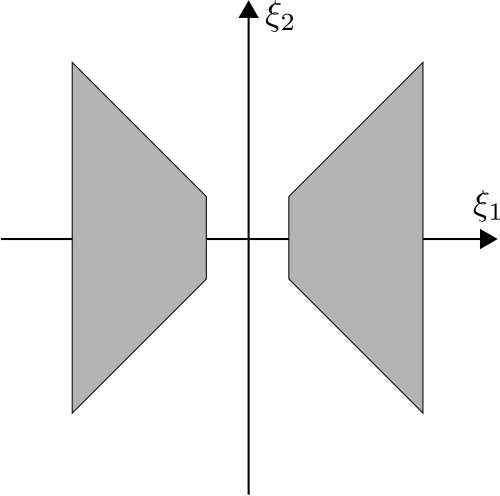
円錐形に適応した小枝 上記のように定義されたシャーレットの欠点の1つは、大きなせん断パラメータに関連するシャーレット要素の方向性バイアスです。この効果は、古典的なシャーレットの周波数タイリングですでに認識されており(セクション#例 の図を参照)、シャーレットの周波数サポートはますます次の方向に整列します。ξ 2 {\displaystyle \xi _{2}} s {\displaystyle s} ξ 2 {\displaystyle \xi _{2}}
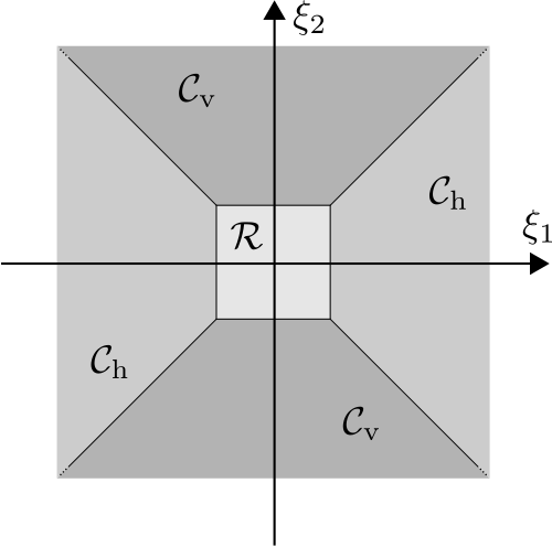
周波数領域を円錐状に分解する。 この問題に対処するため、周波数領域は低周波数部分と2つの円錐領域に分割されます(図を参照)。
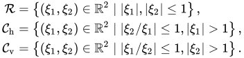
R = { ( ξ 1 、 ξ 2 ) ∈ R 2 ∣ | ξ 1 | 、 | ξ 2 | ≤ 1 } 、 C h = { ( ξ 1 、 ξ 2 ) ∈ R 2 ∣ | ξ 2 / ξ 1 | ≤ 1 、 | ξ 1 | > 1 } 、 C v = { ( ξ 1 、 ξ 2 ) ∈ R 2 ∣ | ξ 1 / ξ 2 | ≤ 1 、 | ξ 2 | > 1 } 。 {\displaystyle {\begin{aligned}{\mathcal {R}}&=\left\{(\xi _{1},\xi _{2})\in \mathbb {R} ^{2}\mid |\xi _{1}|,|\xi _{2}|\leq 1\right\},\\{\mathcal {C}}_{\mathrm {h} }&=\left\{(\xi _{1},\xi _{2})\in \mathbb {R} ^{2}\mid |\xi _{2}/\xi _{1}|\leq 1,|\xi _{1}|>1\right\},\\{\mathcal {C}}_{\mathrm {v} }&=\left\{(\xi _{1},\xi _{2})\in \mathbb {R} ^{2}\mid |\xi _{1}/\xi _{2}|\leq 1,|\xi _{2}|>1\right\}.\end{aligned}}} 古典的なシャーレットによって生成された、円錐適応型シャーレットシステムの周波数タイリング。 関連する円錐適応型離散シャーレットシステムは 3つの部分から構成され、それぞれがこれらの周波数領域の1つに対応しています。これは3つの関数によって生成されます。ϕ 、 ψ 、 ψ ~ ∈ L 2 ( R 2 ) {\displaystyle \phi ,\psi ,{\tilde {\psi }}\in L^{2}(\mathbb {R} ^{2})} サンプリング c = ( c 1 、 c 2 ) ∈ ( R > 0 ) 2 : {\displaystyle c=(c_{1},c_{2})\in (\mathbb {R} _{>0})^{2}:}
SH ( ϕ 、 ψ 、 ψ ~ ; c ) = Φ ( ϕ ; c 1 ) ∪ Ψ ( ψ ; c ) ∪ Ψ ~ ( ψ ~ ; c ) 、 {\displaystyle \operatorname {SH} (\phi ,\psi ,{\tilde {\psi }};c)=\Phi (\phi ;c_{1})\cup \Psi (\psi ;c)\cup {\tilde {\Psi }}({\tilde {\psi }};c),} どこ
Φ ( ϕ ; c 1 ) = { ϕ m = ϕ ( ⋅ − c 1 m ) ∣ m ∈ Z 2 } 、 Ψ ( ψ ; c ) = { ψ j 、 k 、 m = 2 3 j / 4 ψ ( S k A 2 j ⋅ − M c m ) ∣ j ≥ 0 、 | k | ≤ ⌈ 2 j / 2 ⌉ 、 m ∈ Z 2 } 、 Ψ ~ ( ψ ~ ; c ) = { ψ ~ j 、 k 、 m = 2 3 j / 4 ψ ( S ~ k A ~ 2 j ⋅ − M ~ c m ) ∣ j ≥ 0 、 | k | ≤ ⌈ 2 j / 2 ⌉ 、 m ∈ Z 2 } 、 {\displaystyle {\begin{aligned}\Phi (\phi ;c_{1})&=\{\phi _{m}=\phi (\cdot {}-c_{1}m)\mid m\in \mathbb {Z} ^{2}\},\\\Psi (\psi ;c)&=\{\psi _{j,k,m}=2^{3j/4}\psi (S_{k}A_{2^{j}}\cdot {}-M_{c}m)\mid j\geq 0,|k|\leq \lceil 2^{j/2}\rceil ,m\in \mathbb {Z} ^{2}\},\\{\tilde {\Psi }}({\tilde {\psi }};c)&=\{{\tilde {\psi }}_{j,k,m}=2^{3j/4}\psi ({\tilde {S}}_{k}{\tilde {A}}_{2^{j}}\cdot {}-{\tilde {M}}_{c}m)\mid j\geq 0,|k|\leq \lceil 2^{j/2}\rceil ,m\in \mathbb {Z} ^{2}\},\end{aligned}}} と
A ~ 1 = [ 1 1 / 2 0 0 1 ] 、 1 > 0 、 S ~ s = [ 1 0 s 1 ] 、 s ∈ R 、 M c = [ c 1 0 0 c 2 ] 、 そして M ~ c = [ c 2 0 0 c 1 ] 。 {\displaystyle {\begin{aligned}&{\tilde {A}}_{a}={\begin{bmatrix}a^{1/2}&0\\0&a\end{bmatrix}},\;a>0,\quad {\tilde {S}}_{s}={\begin{bmatrix}1&0\\s&1\end{bmatrix}},\;s\in \mathbb {R} ,\quad M_{c}={\begin{bmatrix}c_{1}&0\\0&c_{2}\end{bmatrix}},\quad {\text{and}}\quad {\tilde {M}}_{c}={\begin{bmatrix}c_{2}&0\\0&c_{1}\end{bmatrix}}.\end{aligned}}} システムΨ ( ψ ) {\displaystyle \Psi (\psi )} Ψ ~ ( ψ ~ ) {\displaystyle {\tilde {\Psi }}({\tilde {\psi }})} x 1 {\displaystyle x_{1}} x 2 {\displaystyle x_{2}} C h {\displaystyle {\mathcal {C}}_{\mathrm {h} }} C v {\displaystyle {\mathcal {C}}_{\mathrm {v} }} スケーリング関数 ϕ {\displaystyle \phi } R {\displaystyle {\mathcal {R}}}
参考文献 ↑ Guo, Kanghui、 Gitta Kutyniok 、および Demetrio Labate。「異方性膨張演算子とせん断演算子を使用した疎な多次元表現」。Wavelets and Splines (Athens, GA, 2005)、G. Chen および MJ Lai 編、Nashboro Press、Nashville、TN (2006): 189–201。 「PDF」(PDF) 。 ↑ Donoho, David Leigh. 「画像の疎成分と最適な原子分解」『Constructive Approximation』 17.3 (2001): 353–382. 「PDF」 。CiteSeerX 10.1.1.379.8993 。 ↑ Guo, Kanghui、および Demetrio Labate。「シャーレットを用いた最適スパース多次元表現」SIAM Journal on Mathematical Analysis 39.1 (2007): 298–318。 「PDF」 (PDF) 。 1 2 Kutyniok, Gitta 、および Wang-Q Lim。「コンパクトにサポートされたシャーレットは最適に疎である」。Journal of Approximation Theory 163.11 (2011): 1564–1589。 「PDF」 (PDF) 。 1 2 3 4 5 ギッタ・クティニオク 、デメトリオ・ラバテ編『シアレット:多変量データのためのマルチスケール解析 』Springer、2012年、 ISBN 0-8176-8315-1 ↑ Kittipoom, Pisamai、 Gitta Kutyniok 、および Wang-Q Lim。「コンパクトに支持されたシャーレットフレームの構成」。Constructive Approximation 35.1 (2012): 21–72。Kittipoom , P.; Kutyniok, G.; Lim, W. (2010)。「PDF」。arXiv : 1003.5481 [ math.FA ] 。 1 2 3 Kutyniok, Gitta 、Jakob Lemvig、Wang-Q Lim。「コンパクトにサポートされたシャーレットフレームによる 3D 関数の最適スパース近似」SIAM Journal on Mathematical Analysis 44.4 (2012): 2962–3017。Kutyniok , Gitta; Lemvig, Jakob; Lim, Wang-Q (2011)。「PDF」。arXiv : 1109.5993 [ math.FA ] 。 ↑ Purnendu Banerjee および BB Chaudhuri、「ウェーブレット変換とシャーレット変換を使用したビデオ テキストの局所化」、Proc. SPIE 9021、Document Recognition and Retrieval XXI、2014 年 (doi:10.1117/12.2036077)。 Banerjee、Purnendu; Chaudhuri、BB (2013)。「ウェーブレット変換とシャーレット変換を使用 したビデオ テキスト の 局所化」。Coüasnon、Bertrand; Ringger、Eric K ( 編)。Document Recognition and Retrieval XXI。Vol . 9021。pp. 90210B。arXiv : 1307.4990。doi : 10.1117/12.2036077。S2CID 10659099 。 ↑ Guo, Kanghui、および Demetrio Labate。「シアレットの滑らかなパーセバルフレームの構築」。Mathematical Modelling of Natural Phenomena 8.01 (2013): 82–105。 「PDF」 (PDF) 。 ↑ Grohs, Philipp およびKutyniok, Gitta 。「放物線分子」。Foundations of Computational Mathematics (掲載予定) Grohs, Philipp; Kutyniok, Gitta (2012)。「PDF」。arXiv : 1206.1958 [ math.FA ] 。 ↑ グレン・R・イーズリー;郭康輝。ラバーテ、デメトリオ。パハリ、バサンタ R. (2020-08-10)。 「漫画のような円筒形データの最適なスパース表現」 。 幾何学解析ジャーナル 。 39 (9): 8926–8946 。 土井 : 10.1007/s12220-020-00493-0 。 S2CID 221675372 。 2022-01-22 に取得 。 ↑ Bernhard, Bernhard G.; Labate, Demetrio; Pahari, Basanta R. (2019-10-29). "Smooth projections and the construction of smooth Parseval frames of shearlets" . Advances in Computational Mathematics . 45 ( 5–6 ): 3241–3264 . doi : 10.1007/s10444-019-09736-3 . S2CID 210118010. 2022-01-22 に 取得。
外部リンク ギッタ・クティニオクのホームページ デメトリオ・ラバテのホームページ 




![{\displaystyle [0,1]^{2}}](https://wikimedia.org/api/rest_v1/media/math/render/svg/e2fd6e9b0db782a26c033d7c728aadac9eec363a)















![{\displaystyle \operatorname {supp} {\hat {\psi }}_{1}\subseteq [-{\tfrac {1}{2}},-{\tfrac {1}{16}}]\cup [{\tfrac {1}{16}},{\tfrac {1}{2}}],}](https://wikimedia.org/api/rest_v1/media/math/render/svg/0fd994a790ae83d9e4432998b8e148da9c2c7ba4)


![{\displaystyle \operatorname {supp} {\hat {\psi }}_{2}\subseteq [-1,1]}](https://wikimedia.org/api/rest_v1/media/math/render/svg/4be9d7048ed3022be72a06f098288a848f9feef6)
![\displaystyle \sum _{k=-1}^{1}|{\hat {\psi }}_{2}(\xi +k)|^{2}=1,{\text{ただし、$\xi \in \left[-1,1\right]$。}](https://wikimedia.org/api/rest_v1/media/math/render/svg/2fa08b5c6527adfc7cc1f2651b4b413109730f1e)