代数幾何学 において 、 Quot スキームは、 射影スキーム 上の層をパラメータ化するスキームです 。より具体的には、 X がノイザンスキーム S 上の射影スキームであり 、 F が X 上の 連接層 である場合、 T 点 の集合が T 上で平坦な の 商 の 同型類の集合である スキームが存在します。この概念は 、アレクサンダー・グロタンディーク によって導入されました 。 [1]
引用
ふ
( バツ )
{\displaystyle \operatorname {Quot} _{F}(X)}
引用
ふ
( バツ ) ( T ) =
モア
S
( T 、
引用
ふ
( バツ ) )
{\displaystyle \operatorname {Quot} _{F}(X)(T)=\operatorname {Mor} _{S}(T,\operatorname {Quot} _{F}(X))}
ふ
×
S
T
{\displaystyle F\times _{S}T}
これは通常、ヒルベルト スキーム などの、関心のある幾何学的オブジェクトをパラメーター化する別のスキームを構築するために使用されます 。(実際、 F を 構造層とすると 、ヒルベルト スキームが得られます。)
お
バツ
{\displaystyle {\mathcal {O}}_{X}}
意味 ネーター 基底スキーム 上の 有限型のスキーム と コヒーレント層
に対して 、関手 [2] [3]が存在する。
バツ → S
{\displaystyle X\to S}
S
{\displaystyle S}
え
∈
コー
( バツ )
{\displaystyle {\mathcal {E}}\in {\text{Coh}}(X)}
質問 あなた o t
え
/
バツ
/
S
: ( S c h
/
S
)
o p
→
セット
{\displaystyle {\mathcal {Quot}}_{{\mathcal {E}}/X/S}:(Sch/S)^{op}\to {\text{集合}}}
送信 先
T → S
{\displaystyle T\to S}
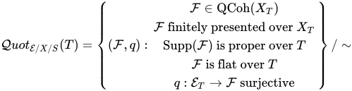
質問 あなた o t
え
/
バツ
/
S
( T ) =
{
(
ふ
、 q ) :
ふ
∈
QCoh
(
バツ
T
)
ふ
有限に提示された
バツ
T
サップ
(
ふ
)
適切です
T
ふ
平らになっている
T
q :
え
T
→
ふ
射影的な
}
/
〜
{\displaystyle {\mathcal {Quot}}_{{\mathcal {E}}/X/S}(T)=\left\{({\mathcal {F}},q):{\begin{matrix}{\mathcal {F}}\in {\text{QCoh}}(X_{T})\\{\mathcal {F}}\ {\text{有限表示}}\ X_{T}\\{\text{Supp}}({\mathcal {F}}){\text{ }}T 上で適切\\{\mathcal {F}}{\text{ }}T 上で平坦\\q:{\mathcal {E}}_{T}\to {\mathcal {F}}{\text{全射}}\end{matrix}}\right\}/\sim }
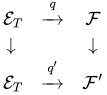
ここで 、 射影 と である。2 つの射影 と可換な 同型が存在する場合、 によって同値関係が与えられる 。つまり、
バツ
T
= バツ
×
S
T
{\displaystyle X_{T}=X\times _{S}T}
え
T
= p
r
バツ
∗
え
{\displaystyle {\mathcal {E}}_{T}=pr_{X}^{*}{\mathcal {E}}}
p
r
バツ
:
バツ
T
→ バツ
{\displaystyle pr_{X}:X_{T}\to X}
(
ふ
、 q ) 〜 (
ふ
′
、
q ′
)
{\displaystyle ({\mathcal {F}},q)\sim ({\mathcal {F}}',q')}
ふ
→
ふ
′
{\displaystyle {\mathcal {F}}\to {\mathcal {F}}'}
q 、
q ′
{\displaystyle q,q'}
え
T
→
q
ふ
↓
↓
え
T
→
q ′
ふ
′
{\displaystyle {\begin{matrix}{\mathcal {E}}_{T}&{\xrightarrow {q}}&{\mathcal {F}}\\\downarrow {}&&\downarrow \\{\mathcal {E}}_{T}&{\xrightarrow {q'}}&{\mathcal {F}}'\end{matrix}}}
は の可換図式です 。あるいは、 が成り立つという同等の条件があります 。これは quot 関手 と呼ばれ、これは部分関手の互いに素な和集合に自然に成層化します。各部分関手はヒルベルト多項式 に関連付けられた quot スキームと呼ばれる射影的 -スキーム によって表されます 。
え
T
→
私 d
え
T
{\displaystyle {\mathcal {E}}_{T}{\xrightarrow {id}}{\mathcal {E}}_{T}}
カー
( q ) =
カー
(
q ′
)
{\displaystyle {\text{ker}}(q)={\text{ker}}(q')}
S
{\displaystyle S}
Φ
{\displaystyle \Phi}
ヒルベルト多項式 比較的非常に豊富な 線束 [4] と任意の 閉点
に対して 、
ら
∈
写真
( バツ )
{\displaystyle {\mathcal {L}}\in {\text{Pic}}(X)}
s ∈ S
{\displaystyle s\in S}
Φ
ふ
:
いいえ
→
いいえ
{\displaystyle \Phi _{\mathcal {F}}:\mathbb {N} \to \mathbb {N} }
メートル ↦ χ (
ふ
s
( メートル ) ) =
∑
私 = 0
ん
( − 1
)
私
薄暗い
κ ( s )
H
私
( バツ 、
ふ
s
⊗
ら
s
⊗ メートル
)
{\displaystyle m\mapsto \chi ({\mathcal {F}}_{s}(m))=\sum _{i=0}^{n}(-1)^{i}{\text{dim }}_{\kappa (s)}H^{i}(X,{\mathcal {F}}_{s}\otimes {\mathcal {L}}_{s}^{\otimes m})}
これは に対する多項式である。これは ヒルベルト多項式 と呼ばれ 、quot 関数の自然な層化を与える。また、 が固定されている場合、部分関数の互いに素な和集合が存在する。
メートル >> 0
{\displaystyle m>>0}
ら
{\displaystyle {\mathcal {L}}}
質問 あなた o t
え
/
バツ
/
S
=
∐
Φ ∈
質問
[ t ]
質問 あなた o t
え
/
バツ
/
S
Φ 、
ら
{\displaystyle {\mathcal {Quot}}_{{\mathcal {E}}/X/S}=\coprod _{\Phi \in \mathbb {Q} [t]}{\mathcal {Quot}}_{{\mathcal {E}}/X/S}^{\Phi ,{\mathcal {L}}}}
どこ
質問 あなた o t
え
/
バツ
/
S
Φ 、
ら
( T ) =
{
(
ふ
、 q ) ∈
質問 あなた o t
え
/
バツ
/
S
( T ) :
Φ
ふ
= Φ
}
{\displaystyle {\mathcal {Quot}}_{{\mathcal {E}}/X/S}^{\Phi ,{\mathcal {L}}}(T)=\left\{({\mathcal { F}},q)\in {\mathcal {Quot}}_{{\mathcal {E}}/X/S}(T):\Phi _{\mathcal {F}}=\ファイ \右\}}
ヒルベルト多項式は、 閉点 に対する のヒルベルト多項式です 。ヒルベルト多項式は、非常に豊富な直線束の選択に依存しないことに注意してください 。
Φ
ふ
{\displaystyle \Phi _{\mathcal {F}}}
ふ
t
{\displaystyle {\mathcal {F}}_{t}}
t ∈ T
{\displaystyle t\in T}
ら
{\displaystyle {\mathcal {L}}}
グロタンディークの存在定理 関数はすべて上の 射影スキームによって表現可能である というのはグロタンディークの定理です 。
質問 あなた o t
え
/
バツ
/
S
Φ 、
ら
{\displaystyle {\mathcal {Quot}}_{{\mathcal {E}}/X/S}^{\Phi ,{\mathcal {L}}}}
引用
え
/
バツ
/
S
Φ
{\displaystyle {\text{Quot}}_{{\mathcal {E}}/X/S}^{\Phi }}
S
{\displaystyle S}
例
グラスマン 次元ベクトル空間の平面の
グラスマン多様体 は 普遍商を持つ
グ ( ん 、 け )
{\displaystyle G(n,k)}
け
{\displaystyle k}
n
{\displaystyle n}
O
G
(
n
,
k
)
⊕
k
→
U
{\displaystyle {\mathcal {O}}_{G(n,k)}^{\oplus k}\to {\mathcal {U}}}
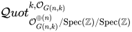
ここで は で表される -平面 です 。は 局所的に自由であり、すべての点で -平面を表すため、定数ヒルベルト多項式 を持ちます 。これは、 が quot 関数を表すことを示しています。
U
x
{\displaystyle {\mathcal {U}}_{x}}
k
{\displaystyle k}
x
∈
G
(
n
,
k
)
{\displaystyle x\in G(n,k)}
U
{\displaystyle {\mathcal {U}}}
k
{\displaystyle k}
Φ
(
λ
)
=
k
{\displaystyle \Phi (\lambda )=k}
G
(
n
,
k
)
{\displaystyle G(n,k)}
Q
u
o
t
O
G
(
n
,
k
)
⊕
(
n
)
/
Spec
(
Z
)
/
Spec
(
Z
)
k
,
O
G
(
n
,
k
)
{\displaystyle {\mathcal {Quot}}_{{\mathcal {O}}_{G(n,k)}^{\oplus (n)}/{\text{Spec}}(\mathbb {Z} )/{\text{Spec}}(\mathbb {Z} )}^{k,{\mathcal {O}}_{G(n,k)}}}
射影空間
特別なケースとして、プロジェクト空間を 「スキーム」として構築することができます。
P
(
E
)
{\displaystyle \mathbb {P} ({\mathcal {E}})}
Q
u
o
t
E
/
X
/
S
1
,
O
X
{\displaystyle {\mathcal {Quot}}_{{\mathcal {E}}/X/S}^{1,{\mathcal {O}}_{X}}}
-scheme 上の 束に対して 。
E
{\displaystyle {\mathcal {E}}}
S
{\displaystyle S}
X
{\displaystyle X}
ヒルベルトスキーム
ヒルベルトスキームは「スキーム」の特別な例です。サブスキームは 射影として与えられることに注意してください。
Z
⊂
X
{\displaystyle Z\subset X}
O
X
→
O
Z
{\displaystyle {\mathcal {O}}_{X}\to {\mathcal {O}}_{Z}}
そして、そのような投影の平坦な族は、スキームによってパラメータ化され、 次のように与えられる。
T
∈
S
c
h
/
S
{\displaystyle T\in Sch/S}
O
X
T
→
F
{\displaystyle {\mathcal {O}}_{X_{T}}\to {\mathcal {F}}}
に関連付けられ たヒルベルト多項式が存在するので 、スキームの同型性が存在する。
Z
{\displaystyle Z}
Φ
Z
{\displaystyle \Phi _{Z}}
Quot
O
X
/
X
/
S
Φ
Z
≅
Hilb
X
/
S
Φ
Z
{\displaystyle {\text{Quot}}_{{\mathcal {O}}_{X}/X/S}^{\Phi _{Z}}\cong {\text{Hilb}}_{X/S}^{\Phi _{Z}}}
パラメータ化の例 代数的に閉じた体
に対して 、非ゼロ断面は ヒルベルト多項式で 消失軌跡を持つ。
X
=
P
k
n
{\displaystyle X=\mathbb {P} _{k}^{n}}
S
=
Spec
(
k
)
{\displaystyle S={\text{Spec}}(k)}
s
∈
Γ
(
O
(
d
)
)
{\displaystyle s\in \Gamma ({\mathcal {O}}(d))}
Z
=
Z
(
s
)
{\displaystyle Z=Z(s)}
Φ
Z
(
λ
)
=
(
n
+
λ
n
)
−
(
n
−
d
+
λ
n
)
{\displaystyle \Phi _{Z}(\lambda )={\binom {n+\lambda }{n}}-{\binom {n-d+\lambda }{n}}}
そして、射影がある
O
→
O
Z
{\displaystyle {\mathcal {O}}\to {\mathcal {O}}_{Z}}
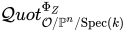
核 を持つ 。 は 任意の非ゼロ断面であり、 に対するの消失軌跡は 同じ消失軌跡を与えるので、 スキームはそのようなすべての断面の自然なパラメータ化を与える。 上に 層があり、 任意の に対して、関連する部分スキーム と全射 が 存在する 。この構成は、quot 関手
O
(
−
d
)
{\displaystyle {\mathcal {O}}(-d)}
s
{\displaystyle s}
a
⋅
s
{\displaystyle a\cdot s}
a
∈
k
∗
{\displaystyle a\in k^{*}}
Q
=
P
(
Γ
(
O
(
d
)
)
)
{\displaystyle Q=\mathbb {P} (\Gamma ({\mathcal {O}}(d)))}
E
{\displaystyle {\mathcal {E}}}
X
×
Q
{\displaystyle X\times Q}
[
s
]
∈
Q
{\displaystyle [s]\in Q}
Z
⊂
X
{\displaystyle Z\subset X}
O
→
O
Z
{\displaystyle {\mathcal {O}}\to {\mathcal {O}}_{Z}}
Q
u
o
t
O
/
P
n
/
Spec
(
k
)
Φ
Z
{\displaystyle {\mathcal {Quot}}_{{\mathcal {O}}/\mathbb {P} ^{n}/{\text{Spec}}(k)}^{\Phi _{Z}}}
射影平面上の二次曲面 かつ
のとき 、ヒルベルト多項式は
X
=
P
2
{\displaystyle X=\mathbb {P} ^{2}}
s
∈
Γ
(
O
(
2
)
)
{\displaystyle s\in \Gamma ({\mathcal {O}}(2))}
Φ
Z
(
λ
)
=
(
2
+
λ
2
)
−
(
2
−
2
+
λ
2
)
=
(
λ
+
2
)
(
λ
+
1
)
2
−
λ
(
λ
−
1
)
2
=
λ
2
+
3
λ
+
2
2
−
λ
2
−
λ
2
=
2
λ
+
2
2
=
λ
+
1
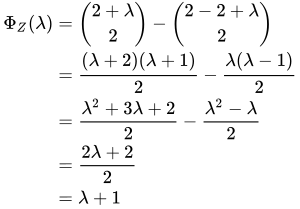
{\displaystyle {\begin{aligned}\Phi _{Z}(\lambda )&={\binom {2+\lambda }{2}}-{\binom {2-2+\lambda }{2}}\\&={\frac {(\lambda +2)(\lambda +1)}{2}}-{\frac {\lambda (\lambda -1)}{2}}\\&={\frac {\lambda ^{2}+3\lambda +2}{2}}-{\frac {\lambda ^{2}-\lambda }{2}}\\&={\frac {2\lambda +2}{2}}\\&=\lambda +1\end{aligned}}}
そして
Quot
O
/
P
2
/
Spec
(
k
)
λ
+
1
≅
P
(
Γ
(
O
(
2
)
)
)
≅
P
5
{\displaystyle {\text{Quot}}_{{\mathcal {O}}/\mathbb {P} ^{2}/{\text{Spec}}(k)}^{\lambda +1}\cong \mathbb {P} (\Gamma ({\mathcal {O}}(2)))\cong \mathbb {P} ^{5}}
上の普遍商は 次のように与えられる。
P
5
×
P
2
{\displaystyle \mathbb {P} ^{5}\times \mathbb {P} ^{2}}
O
→
U
{\displaystyle {\mathcal {O}}\to {\mathcal {U}}}
ここで、点上のファイバーは 射影写像を与える。
[
Z
]
∈
Quot
O
/
P
2
/
Spec
(
k
)
λ
+
1
{\displaystyle [Z]\in {\text{Quot}}_{{\mathcal {O}}/\mathbb {P} ^{2}/{\text{Spec}}(k)}^{\lambda +1}}
O
→
O
Z
{\displaystyle {\mathcal {O}}\to {\mathcal {O}}_{Z}}
例えば、 係数が
[
Z
]
=
[
a
0
:
a
1
:
a
2
:
a
3
:
a
4
:
a
5
]
{\displaystyle [Z]=[a_{0}:a_{1}:a_{2}:a_{3}:a_{4}:a_{5}]}
f
=
a
0
x
2
+
a
1
x
y
+
a
2
x
z
+
a
3
y
2
+
a
4
y
z
+
a
5
z
2
{\displaystyle f=a_{0}x^{2}+a_{1}xy+a_{2}xz+a_{3}y^{2}+a_{4}yz+a_{5}z^{2}}
上の普遍商は、 短い正確な数列を与える。
[
Z
]
{\displaystyle [Z]}
0
→
O
(
−
2
)
→
f
O
→
O
Z
→
0
{\displaystyle 0\to {\mathcal {O}}(-2){\xrightarrow {f}}{\mathcal {O}}\to {\mathcal {O}}_{Z}\to 0}
曲線上の半安定ベクトル束 種数 曲線上の 半安定ベクトル束は 、有限階数の局所自由層として同値に記述できる。このような 階数 と次数の局所自由層は 、以下の性質を持つ [5]。
C
{\displaystyle C}
g
{\displaystyle g}
F
{\displaystyle {\mathcal {F}}}
n
{\displaystyle n}
d
{\displaystyle d}
H
1
(
C
,
F
)
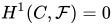
=
0
{\displaystyle H^{1}(C,{\mathcal {F}})=0}
F
{\displaystyle {\mathcal {F}}}
グローバルセクションによって生成される
に対して 。これは全射が存在することを意味する。
d
>
n
(
2
g
−
1
)
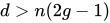
{\displaystyle d>n(2g-1)}
H
0
(
C
,
F
)
⊗
O
C
≅
O
C
⊕
N
→
F
{\displaystyle H^{0}(C,{\mathcal {F}})\otimes {\mathcal {O}}_{C}\cong {\mathcal {O}}_{C}^{\oplus N}\to {\mathcal {F}}}
そして、quotスキームは そのような全射をパラメータ化する。 グロタンディーク・リーマン・ロッホの定理 を用いると、次元 は
Q
u
o
t
O
C
⊕
N
/
C
/
Z
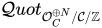
{\displaystyle {\mathcal {Quot}}_{{\mathcal {O}}_{C}^{\oplus N}/{\mathcal {C}}/\mathbb {Z} }}
N
{\displaystyle N}
χ
(
F
)
=
d
+
n
(
1
−
g
)
{\displaystyle \chi ({\mathcal {F}})=d+n(1-g)}
次数の 固定線束には ねじれがあり 、次数が だけシフトするので 、
L
{\displaystyle {\mathcal {L}}}
1
{\displaystyle 1}
F
(
m
)
=
F
⊗
L
⊗
m
{\displaystyle {\mathcal {F}}(m)={\mathcal {F}}\otimes {\mathcal {L}}^{\otimes m}}
n
m
{\displaystyle nm}
χ
(
F
(
m
)
)
=
m
n
+
d
+
n
(
1
−
g
)
{\displaystyle \chi ({\mathcal {F}}(m))=mn+d+n(1-g)}
[5]
ヒルベルト多項式を与える
Φ
F
(
λ
)
=
n
λ
+
d
+
n
(
1
−
g
)
{\displaystyle \Phi _{\mathcal {F}}(\lambda )=n\lambda +d+n(1-g)}
そして、半安定ベクトル束の軌跡は、
Q
u
o
t
O
C
⊕
N
/
C
/
Z
Φ
F
,
L
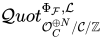
{\displaystyle {\mathcal {Quot}}_{{\mathcal {O}}_{C}^{\oplus N}/{\mathcal {C}}/\mathbb {Z} }^{\Phi _{\mathcal {F}},{\mathcal {L}}}}
これはGIT商 を用いて半安定ベクトル束の モジュライ空間を構築するために使用できる 。 [5]
M
C
(
n
,
d
)
{\displaystyle {\mathcal {M}}_{C}(n,d)}
参照
参考文献
^ グロタンディーク、アレクサンダー。幾何学的計算における構築と存在の技術 IV : ヒルベルトのスキーマ。ブルバキセミナー: années 1960/61、exposés 205-222、Séminaire Bourbaki、no. 6 (1961)、トーク no. 221、p. 249-276 ^ Nitsure, Nitin (2005). 「ヒルベルトおよびクォートスキームの構築」。 基礎代数幾何学: グロタンディークの FGA の説明 。 数学サーベイおよびモノグラフ。 第 123 巻。 アメリカ数学会。 pp. 105–137。 arXiv : math/0504590 。 ISBN 978-0-8218-4245-4 。 ^ Altman, Allen B.; Kleiman, Steven L. (1980). 「Picardスキームのコンパクト化」. Advances in Mathematics . 35 (1): 50–112. doi : 10.1016/0001-8708(80)90043-2 . ISSN 0001-8708. ^ グローバルセクションの 基底は、 埋め込み を定義することを意味します
s
i
{\displaystyle s_{i}}
Γ
(
X
,
L
)
{\displaystyle \Gamma (X,{\mathcal {L}})}
s
:
X
→
P
S
N
{\displaystyle \mathbb {s} :X\to \mathbb {P} _{S}^{N}}
N
=
dim
(
Γ
(
X
,
L
)
)
{\displaystyle N={\text{dim}}(\Gamma (X,{\mathcal {L}}))}
^ abc Hoskins, Victoria. 「モジュライ問題と幾何学的不変理論」 (PDF) 。pp. 68, 74–85。 2020年3月1日時点のオリジナルよりアーカイブ (PDF) 。
さらに読む 安定写像と量子コホモロジーに関するノート https://amathew.wordpress.com/2012/06/02/the-stack-of-coherent-sheaves/ 



















![{\displaystyle {\mathcal {Quot}}_{{\mathcal {E}}/X/S}=\coprod _{\Phi \in \mathbb {Q} [t]}{\mathcal {Quot}}_{{\mathcal {E}}/X/S}^{\Phi ,{\mathcal {L}}}}](https://wikimedia.org/api/rest_v1/media/math/render/svg/f890abd582faea3b13b26c15096e25304eb3b203)













![{\displaystyle [s]\in Q}](https://wikimedia.org/api/rest_v1/media/math/render/svg/1cf2786e0f5d8b3c950b2678cabcd9d655d7e58e)





![{\displaystyle [Z]\in {\text{Quot}}_{{\mathcal {O}}/\mathbb {P} ^{2}/{\text{Spec}}(k)}^{\lambda +1}}](https://wikimedia.org/api/rest_v1/media/math/render/svg/619ebb2770e2fb2e4775cef50709a87c612630c0)
![{\displaystyle [Z]=[a_{0}:a_{1}:a_{2}:a_{3}:a_{4}:a_{5}]}](https://wikimedia.org/api/rest_v1/media/math/render/svg/fd234c33c5c4c4fe1cc483b4f24e2f894b182640)

![{\displaystyle [Z]}](https://wikimedia.org/api/rest_v1/media/math/render/svg/dba10cc2996611bf99b91bbb1c8c22aa504cdfe7)