クラトフスキー閉包公理

位相幾何学や数学の関連分野において、クラトフスキー閉包公理は、集合上の位相構造を定義するために使用できる公理の集合である。これらは、より一般的に使用される開集合の定義と同等である。これらは、カジミエシュ・クラトフスキー^[1]によって最初に形式化され、そのアイデアは、ヴァツワフ・シェルピンスキやアントニオ・モンテイロ^[2]などの数学者によってさらに研究された。

同様の公理セットは、内部演算子の双対概念のみを使用して位相構造を定義するために使用することができます。^[3]

を任意の集合とし、その冪集合をとします。クラトフスキー閉包演算子は、次の特性を持つ 単項演算です。${\displaystyle X}$${\displaystyle \wp (X)}$ ${\displaystyle \mathbf {c} :\wp (X)\to \wp (X)}$

[K1]空集合を保存します: ; ${\displaystyle \mathbf {c} (\varnothing )=\varnothing }$

[K2]それは広範である：すべての に対して、； ${\displaystyle A\subseteq X}$${\displaystyle A\subseteq \mathbf {c} (A)}$

[K3]はべき等性がある：すべての に対して、である。 ${\displaystyle A\subseteq X}$${\displaystyle \mathbf {c} (A)=\mathbf {c} (\mathbf {c} (A))}$

[K4]二項和集合上で保存/分配します。すべての に対して、です。${\displaystyle A,B\subseteq X}$${\displaystyle \mathbf {c} (A\cup B)=\mathbf {c} (A)\cup \mathbf {c} (B)}$

二項和集合を保存することによって、次の条件が成立する: ^[4]${\displaystyle \mathbf {c} }$

[K4']単調です：。${\displaystyle A\subseteq B\Rightarrow \mathbf {c} (A)\subseteq \mathbf {c} (B)}$

実際、[K4]の等式を包含として書き直すと、より弱い公理[K4'']（劣加法性）が得られます。

[K4'']劣加法性がある：すべての、、に対して${\displaystyle A,B\subseteq X}$${\displaystyle \mathbf {c} (A\cup B)\subseteq \mathbf {c} (A)\cup \mathbf {c} (B)}$

すると、公理[K4']と[K4'']を合わせると[K4]と同等であることが簡単に分かります（以下の証明2の最後から2番目の段落を参照）。

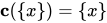
クラトフスキー (1966) は、単一集合が閉包に関して安定でなければならないことを要求する第 5 の (オプションの) 公理を含めています。これは、すべての に対して、です。彼は、5 つの公理すべてを満たす位相空間を、挙げられている 4 つの公理のみを満たすより一般的な空間とは対照的に、 T ₁空間と呼んでいます。実際、これらの空間は通常の対応関係によって位相 T ₁空間と正確に対応しています(以下を参照)。^[5]${\displaystyle x\in X}$${\displaystyle \mathbf {c} (\{x\})=\{x\}}$

要件[K3]が省略された場合、公理はČech閉包演算子を定義します。^{[6]代わりに}[K1]が省略された場合、[K2]、[K3]、[K4']を満たす演算子はムーア閉包演算子と呼ばれます。^[7]ペアは、が満たす公理に応じて、クラトフスキー閉包空間、Čech閉包空間、またはムーア閉包空間と呼ばれます。 ${\displaystyle (X,\mathbf {c} )}$${\displaystyle \mathbf {c} }$

4つのクラトフスキー閉包公理は、パーヴィンによって与えられた1つの条件に置き換えることができる。^[8]

[P]すべての について、。${\displaystyle A,B\subseteq X}$${\displaystyle A\cup \mathbf {c} (A)\cup \mathbf {c} (\mathbf {c} (B))=\mathbf {c} (A\cup B)\setminus \mathbf {c} (\varnothing )}$

この要件の結果として 公理[K1] - [K4]を導くことができる。

1. を選択してください。次に、 または を選択します。これは直ちに[K1]を意味します。${\displaystyle A=B=\varnothing }$${\displaystyle \varnothing \cup \mathbf {c} (\varnothing )\cup \mathbf {c} (\mathbf {c} (\varnothing ))=\mathbf {c} (\varnothing )\setminus \mathbf {c} (\varnothing )=\varnothing }$${\displaystyle \mathbf {c} (\varnothing )\cup \mathbf {c} (\mathbf {c} (\varnothing ))=\varnothing }$
2. 任意のと を選択します。次に、公理[K1]、を適用して、[K2]を意味します。${\displaystyle A\subseteq X}$${\displaystyle B=\varnothing }$${\displaystyle A\cup \mathbf {c} (A)=\mathbf {c} (A)}$
3. と任意のを選択する。次に、公理[K1]を適用すると、となり、これは[K3]となる。${\displaystyle A=\varnothing }$${\displaystyle B\subseteq X}$${\displaystyle \mathbf {c} (\mathbf {c} (B))=\mathbf {c} (B)}$
4. 任意の を選択する。公理[K1] – [K3]を適用すると、[K4]が導出される。${\displaystyle A,B\subseteq X}$

あるいは、モンテイロ（1945）は、 [K2] – [K4]のみを伴うより弱い公理を提案した：^[9]

[M]すべての について、.${\displaystyle A,B\subseteq X}$${\textstyle A\cup \mathbf {c} (A)\cup \mathbf {c} (\mathbf {c} (B))\subseteq \mathbf {c} (A\cup B)}$

要件[K1] は[M]とは独立しています 。実際、 の場合、定数割り当てによって定義される演算子は[M]を満たしますが、 であるため、空集合は保存されません。定義により、[M] を満たす演算子はすべてムーア閉包演算子であることに注意してください。 ${\displaystyle X\neq \varnothing }$${\displaystyle \mathbf {c} ^{\star }:\wp (X)\to \wp (X)}$${\displaystyle A\mapsto \mathbf {c} ^{\star }(A):=X}$${\displaystyle \mathbf {c} ^{\star }(\varnothing )=X}$

[M]のより対称的な代替案もMO BotelhoとMH Teixeiraによって証明され、公理[K2] - [K4]が導かれる: ^[2]

[BT]すべての について、。${\displaystyle A,B\subseteq X}$${\textstyle A\cup B\cup \mathbf {c} (\mathbf {c} (A))\cup \mathbf {c} (\mathbf {c} (B))=\mathbf {c} (A\cup B)}$

クラトフスキー閉包作用素の双対概念としてクラトフスキー内部作用素があり、これは次のような類似の要件を満たす写像である: ^[3]${\displaystyle \mathbf {i} :\wp (X)\to \wp (X)}$

[I1]総スペースが維持されます: ; ${\displaystyle \mathbf {i} (X)=X}$

[I2]それは強意的である：すべての に対して、； ${\displaystyle A\subseteq X}$${\displaystyle \mathbf {i} (A)\subseteq A}$

[I3]これは冪等である: すべての に対して、 である; ${\displaystyle A\subseteq X}$${\displaystyle \mathbf {i} (\mathbf {i} (A))=\mathbf {i} (A)}$

[I4]二項共通集合が保存される：すべての に対して、。${\displaystyle A,B\subseteq X}$${\displaystyle \mathbf {i} (A\cap B)=\mathbf {i} (A)\cap \mathbf {i} (B)}$

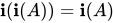
これらの演算子については、クラトフスキー閉包について推論されたものと完全に類似した結論に達することができます。たとえば、すべてのクラトフスキー内部演算子は等価です。つまり、 [K4']を満たし、強度[I2]により、 [I3]の等式を単純な包含に弱めることが可能です。

クラトフスキー閉包と内部空間の双対性は、上の自然補数演算子によって提供され、写像はを送る。この写像は冪集合格子上の直交補写像であり、ド・モルガンの法則を満たす。 が任意の添字集合で である場合、 ${\displaystyle \wp (X)}$${\displaystyle \mathbf {n} :\wp (X)\to \wp (X)}$${\displaystyle A\mapsto \mathbf {n} (A):=X\setminus A}$${\displaystyle {\mathcal {I}}}$${\displaystyle \{A_{i}\}_{i\in {\mathcal {I}}}\subseteq \wp (X)}$$${\displaystyle \mathbf {n} \left(\bigcup _{i\in {\mathcal {I}}}A_{i}\right)=\bigcap _{i\in {\mathcal {I}}}\mathbf {n} (A_{i}),\qquad \mathbf {n} \left(\bigcap _{i\in {\mathcal {I}}}A_{i}\right)=\bigcup _{i\in {\mathcal {I}}}\mathbf {n} (A_{i}).}$$

これらの法則を の定義特性とともに用いることで、定義関係(および) を介して、任意のクラトフスキー内部がクラトフスキー閉包を誘導すること (およびその逆) を示すことができます。 に関して得られたすべての結果は、これらの関係を正規補完 の特性と組み合わせて用いることで、に関する結果に変換できます。 ${\displaystyle \mathbf {n} }$${\displaystyle \mathbf {c} :=\mathbf {nin} }$${\displaystyle \mathbf {i} :=\mathbf {ncn} }$${\displaystyle \mathbf {c} }$${\displaystyle \mathbf {i} }$${\displaystyle \mathbf {n} }$

パービン（1964）はさらにクラトフスキー外部演算子^[3]とクラトフスキー境界演算子^[10]に対して類似の公理を与えており、これもまた関係とを介してクラトフスキー閉包を誘導する。 ${\displaystyle \mathbf {c} :=\mathbf {ne} }$${\displaystyle \mathbf {c} (A):=A\cup \mathbf {b} (A)}$

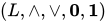
公理[K1] – [K4]は、集合論的包含を格子に関連付けられた半順序に、集合論的和を結合演算に、集合論的積を会合演算に形式的に置き換えることによって、一般有界格子上の抽象的な単項演算を定義するために適応できることに注意されたい。公理[I1] – [I4]についても同様である。格子が直交補集合である場合、これら 2 つの抽象演算は通常の方法で互いを誘導する。抽象閉包または内部演算子は、格子上の 一般化された位相を定義するために使用できる。${\displaystyle \mathbf {c} :L\to L}$${\displaystyle (L,\land ,\lor ,\mathbf {0} ,\mathbf {1} )}$

ムーア閉包演算子の要件には結合も空集合も現れないため、定義は任意のposet上の抽象単項演算子を定義するように適応される可能性があります。 ${\displaystyle \mathbf {c} :S\to S}$ ${\displaystyle S}$

閉包演算子は、次のように自然に位相を誘導します。を任意の集合とします。部分集合がクラトフスキー閉包演算子に関して閉じている場合、それはその演算子の不動点である場合、つまり の下で安定している場合、つまり の場合に限ります。主張は、閉集合の補集合である全体空間の部分集合のすべての族が位相の 3 つの通常の要件を満たす、または同等に、すべての閉集合の族が以下を満たすというものです。 ${\displaystyle X}$${\displaystyle C\subseteq X}$${\displaystyle \mathbf {c} :\wp (X)\to \wp (X)}$ ${\displaystyle \mathbf {c} }$${\displaystyle \mathbf {c} (C)=C}$${\displaystyle {\mathfrak {S}}[\mathbf {c} ]}$

[T1]これはの有界部分格子、すなわち である。 ${\displaystyle \wp (X)}$${\displaystyle X,\varnothing \in {\mathfrak {S}}[\mathbf {c} ]}$

[T2]任意の交差に関して完全である、すなわち、 が任意の添え字の集合であり である場合、 である。 ${\displaystyle {\mathcal {I}}}$${\displaystyle \{C_{i}\}_{i\in {\mathcal {I}}}\subseteq {\mathfrak {S}}[\mathbf {c} ]}$${\textstyle \bigcap _{i\in {\mathcal {I}}}C_{i}\in {\mathfrak {S}}[\mathbf {c} ]}$

[T3]有限和に関して完全である、すなわち、が添え字の有限集合であり、である場合、である。${\displaystyle {\mathcal {I}}}$${\displaystyle \{C_{i}\}_{i\in {\mathcal {I}}}\subseteq {\mathfrak {S}}[\mathbf {c} ]}$${\textstyle \bigcup _{i\in {\mathcal {I}}}C_{i}\in {\mathfrak {S}}[\mathbf {c} ]}$

冪等性[K3]により、簡潔に と書くことができることに注意してください。 ${\displaystyle {\mathfrak {S}}[\mathbf {c} ]=\operatorname {im} (\mathbf {c} )}$

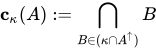
逆に、公理[T1] – [T3]を満たす族が与えられた場合、次のようにクラトフスキー閉包作用素を構成することが可能である。およびがの包含反転である場合、 ${\displaystyle \kappa }$${\displaystyle A\in \wp (X)}$${\displaystyle A^{\uparrow }=\{B\in \wp (X)\ |\ A\subseteq B\}}$${\displaystyle A}$$${\displaystyle \mathbf {c} _{\kappa }(A):=\bigcap _{B\in (\kappa \cap A^{\uparrow })}B}$$

は 上のクラトフスキー閉包演算子を定義します。 ${\displaystyle \mathbf {c} _{\kappa }}$${\displaystyle \wp (X)}$

実際、これら 2 つの補完的な構成は互いに逆です。 が上のすべてのクラトフスキー閉包演算子の集合であり、 が位相内のすべての集合の補集合からなるすべての族の集合、つまり[T1] – [T3]を満たすすべての族の集合である場合、は一対一であり、その逆は割り当て によって与えられます。 ${\displaystyle \mathrm {Cls} _{\text{K}}(X)}$${\displaystyle X}$${\displaystyle \mathrm {Atp} (X)}$${\displaystyle {\mathfrak {S}}:\mathrm {Cls} _{\text{K}}(X)\to \mathrm {Atp} (X)}$${\displaystyle \mathbf {c} \mapsto {\mathfrak {S}}[\mathbf {c} ]}$${\displaystyle {\mathfrak {C}}:\kappa \mapsto \mathbf {c} _{\kappa }}$

また、全単射を を含むすべての Čech 閉包演算子の集合に拡張できることに留意してください。この拡張は全射でもあり、これは 上のすべての Čech 閉包演算子が上にも位相を誘導することを意味します。^[11]しかし、これは がもはや全単射ではない ことを意味します。${\displaystyle {\mathfrak {S}}}$${\displaystyle \mathrm {Cls} _{\check {C}}(X)}$${\displaystyle \mathrm {Cls} _{\text{K}}(X)}$${\displaystyle {\overline {\mathfrak {S}}}}$${\displaystyle X}$${\displaystyle X}$${\displaystyle {\overline {\mathfrak {S}}}}$

• 上で議論したように、位相空間が与えられれば、任意の部分集合の閉包を集合、つまり を含むすべての閉集合の共通部分として定義できます。集合 はを含む最小の閉集合であり、演算子 はクラトフスキー閉包演算子です。${\displaystyle X}$${\displaystyle A\subseteq X}$${\displaystyle \mathbf {c} (A)=\bigcap \{C{\text{ a closed subset of }}X|A\subseteq C\}}$${\displaystyle X}$${\displaystyle A}$${\displaystyle \mathbf {c} (A)}$${\displaystyle X}$${\displaystyle A}$${\displaystyle \mathbf {c} :\wp (X)\to \wp (X)}$
• が任意の集合である場合、となる演算子はクラトフスキー閉包です。最初の演算子は非離散位相 を誘導し、2 番目の演算子は離散位相を誘導します。${\displaystyle X}$${\displaystyle \mathbf {c} _{\top },\mathbf {c} _{\bot }:\wp (X)\to \wp (X)}$$${\displaystyle \mathbf {c} _{\top }(A)={\begin{cases}\varnothing &A=\varnothing ,\\X&A\neq \varnothing ,\end{cases}}\qquad \mathbf {c} _{\bot }(A)=A\quad \forall A\in \wp (X),}$$ ${\displaystyle \{\varnothing ,X\}}$ ${\displaystyle \wp (X)}$

• 任意の を固定し、 がすべての に対してとなるようにします。すると、 はクラトフスキー閉包を定義します。対応する閉集合の族は（を含むすべての部分集合の族）と一致します。 のとき、再び離散位相（つまり、定義からわかるように ）を取得します。${\displaystyle S\subsetneq X}$${\displaystyle \mathbf {c} _{S}:\wp (X)\to \wp (X)}$${\displaystyle \mathbf {c} _{S}(A):=A\cup S}$${\displaystyle A\in \wp (X)}$${\displaystyle \mathbf {c} _{S}}$${\displaystyle {\mathfrak {S}}[\mathbf {c} _{S}]}$${\displaystyle S^{\uparrow }}$${\displaystyle S}$${\displaystyle S=\varnothing }$${\displaystyle \wp (X)}$${\displaystyle \mathbf {c} _{\varnothing }=\mathbf {c} _{\bot }}$
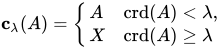
• が となる無限基数である場合、 となる演算子は4 つのクラトフスキー公理をすべて満たします。^[12]の場合、この演算子は上にコ有限位相を誘導します。の場合、コ可算位相を誘導します。${\displaystyle \lambda }$${\displaystyle \lambda \leq \operatorname {crd} (X)}$${\displaystyle \mathbf {c} _{\lambda }:\wp (X)\to \wp (X)}$$${\displaystyle \mathbf {c} _{\lambda }(A)={\begin{cases}A&\operatorname {crd} (A)<\lambda ,\\X&\operatorname {crd} (A)\geq \lambda \end{cases}}}$$${\displaystyle \lambda =\aleph _{0}}$${\displaystyle X}$${\displaystyle \lambda =\aleph _{1}}$

• 任意のクラトフスキー閉包は等長であり、また任意の包含写像も明らかに等長であるため、 を包含に関する半集合として、またのサブ半集合として見れば、 (等長)ガロア接続 が得られます。実際、すべてのおよびに対して、である場合に限り、 であることが簡単に確認できます。${\displaystyle \langle \mathbf {c} :\wp (X)\to \mathrm {im} (\mathbf {c} );\iota :\mathrm {im} (\mathbf {c} )\hookrightarrow \wp (X)\rangle }$${\displaystyle \wp (X)}$${\displaystyle \mathrm {im} (\mathbf {c} )}$${\displaystyle \wp (X)}$${\displaystyle A\in \wp (X)}$${\displaystyle C\in \mathrm {im} (\mathbf {c} )}$${\displaystyle \mathbf {c} (A)\subseteq C}$${\displaystyle A\subseteq \iota (C)}$
• がのサブファミリーである場合、${\displaystyle \{A_{i}\}_{i\in {\mathcal {I}}}}$${\displaystyle \wp (X)}$$${\displaystyle \bigcup _{i\in {\mathcal {I}}}\mathbf {c} (A_{i})\subseteq \mathbf {c} \left(\bigcup _{i\in {\mathcal {I}}}A_{i}\right),\qquad \mathbf {c} \left(\bigcap _{i\in {\mathcal {I}}}A_{i}\right)\subseteq \bigcap _{i\in {\mathcal {I}}}\mathbf {c} (A_{i}).}$$
• もしならば。${\displaystyle A,B\in \wp (X)}$${\displaystyle \mathbf {c} (A)\setminus \mathbf {c} (B)\subseteq \mathbf {c} (A\setminus B)}$

すべての に対してとなるクラトフスキー閉包のペアは、となる位相を誘導し、逆もまた同様です。言い換えると、が優勢となるのは、後者によって誘導される位相が前者によって誘導される位相の精緻化である場合、または同等にである場合に限ります。^[13]たとえば、 は明らかに優勢です(後者は 上の恒等式に過ぎません)。 をそのメンバーすべての補集合を含む族に置き換えても同じ結論に達することができるため、 がすべての に対して半順序を持ち、 が精緻化順序を持つ場合、 は半順序集合間の反調写像であると結論付けることができます。 ${\displaystyle \mathbf {c} _{1},\mathbf {c} _{2}:\wp (X)\to \wp (X)}$${\displaystyle \mathbf {c} _{2}(A)\subseteq \mathbf {c} _{1}(A)}$${\displaystyle A\in \wp (X)}$${\displaystyle \tau _{1},\tau _{2}}$${\displaystyle \tau _{1}\subseteq \tau _{2}}$${\displaystyle \mathbf {c} _{1}}$${\displaystyle \mathbf {c} _{2}}$${\displaystyle {\mathfrak {S}}[\mathbf {c} _{1}]\subseteq {\mathfrak {S}}[\mathbf {c} _{2}]}$${\displaystyle \mathbf {c} _{\top }}$${\displaystyle \mathbf {c} _{\bot }}$${\displaystyle \wp (X)}$${\displaystyle \tau _{i}}$${\displaystyle \kappa _{i}}$${\displaystyle \mathrm {Cls} _{\text{K}}(X)}$${\displaystyle \mathbf {c} \leq \mathbf {c} '\iff \mathbf {c} (A)\subseteq \mathbf {c} '(A)}$${\displaystyle A\in \wp (X)}$${\displaystyle \mathrm {Atp} (X)}$${\displaystyle {\mathfrak {S}}}$

任意の誘導位相（部分集合Aを基準として）において、閉集合は、すべてのに対して、A :に制限された元の閉包演算子である新しい閉包演算子を誘導します。^[14]${\displaystyle \mathbf {c} _{A}(B)=A\cap \mathbf {c} _{X}(B)}$${\displaystyle B\subseteq A}$

関数が点において連続であるためにはが成り立ち、あらゆる部分集合において連続であるためには が成り立つことがその時に限る。^[15]写像が閉写像であるためには逆包含が成り立つことがその時に限る。 ^[16]同相写像であるためには連続かつ閉写像であるため、すなわち等式が成り立つことがその時に限る。^[17]${\displaystyle f:(X,\mathbf {c} )\to (Y,\mathbf {c} ')}$${\displaystyle p}$${\displaystyle p\in \mathbf {c} (A)\Rightarrow f(p)\in \mathbf {c} '(f(A))}$$${\displaystyle f(\mathbf {c} (A))\subseteq \mathbf {c} '(f(A))}$$${\displaystyle A\in \wp (X)}$${\displaystyle f}$

をクラトフスキー閉包空間と する。すると${\displaystyle (X,\mathbf {c} )}$

• ${\displaystyle X}$がT ₀空間である場合、その場合のみ、が成り立つ。^[18]${\displaystyle x\neq y}$${\displaystyle \mathbf {c} (\{x\})\neq \mathbf {c} (\{y\})}$
• ${\displaystyle X}$はT ₁空間であるためにはすべての に対してその限りではない；^[19]${\displaystyle \mathbf {c} (\{x\})=\{x\}}$${\displaystyle x\in X}$
• ${\displaystyle X}$がT ₂空間である場合、かつが存在する場合と同値である。ここで は集合補集合演算子である。^[20]${\displaystyle x\neq y}$${\displaystyle A\in \wp (X)}$${\displaystyle x\notin \mathbf {c} (A)}$${\displaystyle y\notin \mathbf {c} (\mathbf {n} (A))}$${\displaystyle \mathbf {n} }$

ある点が部分集合に近い場合、これは集合の点と部分集合の近接関係を定義するために使用できる。 ^[21]${\displaystyle p}$${\displaystyle A}$${\displaystyle p\in \mathbf {c} (A).}$

二つの集合が分離しているとは、そのときに限ります。空間が連結しているとは、二つの分離された部分集合の和集合として表すことができないときに限られます。^[22]${\displaystyle A,B\in \wp (X)}$${\displaystyle (A\cap \mathbf {c} (B))\cup (B\cap \mathbf {c} (A))=\varnothing }$${\displaystyle X}$

• 位相空間のカテゴリの特徴
• Čech 閉包演算子 – 閉包演算子Pages displaying short descriptions of redirect targets
• 閉包演算子 – 数学演算子Pages displaying wikidata descriptions as a fallback
• 閉包代数 – 代数構造
• 前閉包演算子 – 閉包演算子
• 前位相空間 – 一般化された位相空間
• 位相空間 – 近さの概念を持つ数学的空間

• Kuratowski, Kazimierz (1922) [1920]、「Sur l'opération A de l'Analysis Situs」[分析現場での操作 A について] (PDF)、Fundamenta Mathematicae (フランス語)、vol. 3、182–199ページ。
• クラトフスキー、カジミェシュ(1966) [1958]、トポロジー、vol. I、Jawrowski, J. 訳、Academic Press、ISBN 0-12-429201-1、LCCN  66029221。
  • —— (2010). 「Operation Ā Analysis Situsについて」。ResearchGate。Mark Bowronによる翻訳。
• パービン、ウィリアム J. (1964)、ボアス、ラルフ P. Jr. (編)、一般位相幾何学の基礎、アカデミック プレス、ISBN 9781483225159、LCCN  64-17796。
• アルカンゲルスキー、AV;フェドルチュク、VV (1990) [1988]、ガムクレリゼ、RV。アルカンゲルスキー、AV; Pontryagin、LS (編)、General Topology I、Encyclopedia of Mathematical Sciences、vol. 17、O'Shea 翻訳、DB、ベルリン: Springer-Verlag、ISBN 978-3-642-64767-3、LCCN  89-26209。
• Monteiro, António (1945)、「Caractérisation de l'opération de fermeture par un seul axiome」[単一公理による閉包演算の特徴付け]、Portugaliae mathematica (フランス語)、vol. 4、いいえ。 4、158 ～ 160 ページ、MR  0012310、Zbl  0060.39406。

• 位相空間の代替的な特徴づけ