混合容量

数学、より具体的には凸幾何学において、混合体積は凸体の組に非負の数を関連付ける方法である。$\displaystyle \mathbb {R} ^{n}}$この数は、物体の大きさや形状、そしてそれらの相対的な向きによって異なります。

させて${\displaystyle K_{1},K_{2},\dots ,K_{r}}$凸体である$\displaystyle \mathbb {R} ^{n}}$そして関数を考える

${\displaystyle f(\lambda _{1},\ldots ,\lambda _{r})=\mathrm {Vol} _{n}(\lambda _{1}K_{1}+\cdots +\lambda _{r}K_{r}),\qquad \lambda _{i}\geq 0,}$

どこ${\displaystyle {\text{Vol}}_{n}}$は${\displaystyle n}$次元体積であり、その引数はスケーリングされた凸体のミンコフスキー和である。${\displaystyle K_{i}}$示すことができるのは${\displaystyle f}$次数が の同次多項式である${\displaystyle n}$なので、次のように書くことができます。

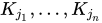
${\displaystyle f(\lambda _{1},\ldots ,\lambda _{r})=\sum _{j_{1},\ldots ,j_{n}=1}^{r}V(K_{j_{1}},\ldots ,K_{j_{n}})\lambda _{j_{1}}\cdots \lambda _{j_{n}},}$

関数${\displaystyle V}$対称です。特定のインデックス関数の場合${\displaystyle j\in \{1,\ldots ,r\}^{n}}$係数${\displaystyle V(K_{j_{1}},\dots ,K_{j_{n}})}$混合体積と呼ばれる${\displaystyle K_{j_{1}},\dots ,K_{j_{n}}}$。

• 混合体積は、以下の3つの特性によって一意に決定されます。

1. ${\displaystyle V(K,\dots ,K)={\text{Vol}}_{n}(K)}$;
2. ${\displaystyle V}$引数に関して対称である。
3. ${\displaystyle V}$多線形です:${\displaystyle V(\lambda K+\lambda 'K',K_{2},\dots ,K_{n})=\lambda V(K,K_{2},\dots ,K_{n})+\lambda 'V(K',K_{2},\dots ,K_{n})}$のために${\displaystyle \lambda ,\lambda '\geq 0}$。

• 混合体積は、各変数に関して非負かつ単調増加する。${\displaystyle V(K_{1},K_{2},\ldots ,K_{n})\leq V(K_{1}',K_{2},\ldots ,K_{n})}$のために${\displaystyle K_{1}\subseteq K_{1}'}$。
• アレクサンドル・ダニロヴィチ・アレクサンドロフとヴェルナー・フェンケルによって発見されたアレクサンドロフとフェンシェルの不等式：

$\displaystyle V(K_{1},K_{2},K_{3},\ldots ,K_{n})\geq \sqrt {V(K_{1},K_{1},K_{3},\ldots ,K_{n})V(K_{2},K_{2},K_{3},\ldots ,K_{n})}}.}$

凸体に対するブルン・ミンコフスキーの不等式やミンコフスキーの第一不等式など、数多くの幾何学的不等式は、アレクサンドロフ・フェンシェルの不等式の特殊な場合である。

させて$\displaystyle K\subset \mathbb {R} ^{n}}$凸体とし、${\displaystyle B=B_{n}\subset \mathbb {R} ^{n}}$単位半径のユークリッド球とする。混合体積

${\displaystyle W_{j}(K)=V({\overset {nj回}}}{\overbrace {K,K,\ldots ,K} }},{\overset {j回}}}{\overbrace {B,B,\ldots ,B} }})}$

は、 j番目のクエルマス積分と呼ばれます。${\displaystyle K}$[ ^{1 ]​}

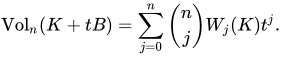
混合体積の定義から、シュタイナーの公式（ヤコブ・シュタイナーにちなんで命名）が得られる。

${\displaystyle \mathrm {Vol} _{n}(K+tB)=\sum _{j=0}^{n}{\binom {n}{j}}W_{j}(K)t^{j}.}$

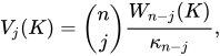
The intrinsic volumes of ${\displaystyle B^{n}}$, the unit ball in ${\displaystyle \mathbb {R} ^{n}}$, satisfy$${\displaystyle {\begin{aligned}&V_{j}\left(B^{n}\right)={\frac {\kappa _{n}}{\kappa _{n-j}}}{\binom {n}{j}},\quad j=0,\ldots ,n.\\&\kappa _{m}=\operatorname {Vol} _{m}\left(B^{m}\right)={\frac {\pi ^{m/2}}{\Gamma \left({\frac {m}{2}}+1\right)}}\end{aligned}}}$$Given an n-dimensional convex body ${\textstyle K}$, the ${\textstyle j}$-th intrinsic volume of ${\textstyle K}$ satisfies the Cauchy-Kubota formula^[3]$${\displaystyle V_{j}(K):={\frac {\kappa _{n}}{\kappa _{j}\kappa _{n-j}}}{\binom {n}{j}}\int _{\mathrm {G} (n,j)}V_{j}\left(\operatorname {proj} _{E}K\right)\mathrm {d} E}$$Here, ${\textstyle \kappa _{j}}$ denotes the ${\textstyle j}$-dimensional volume of the ${\textstyle j}$-dimensional unit ball, integration is with respect to the Haar probability measure on ${\textstyle \mathrm {G} (n,j)}$, the Grassmannian of ${\textstyle j}$-dimensional subspaces in ${\textstyle \mathbb {R} ^{n}}$, and ${\textstyle \operatorname {proj} _{E}:\mathbb {R} ^{n}\rightarrow E}$ denotes the orthogonal projection onto ${\textstyle E\in \mathrm {G} (n,j)}$.

Burago, Yu.D. (2001) [1994], "Mixed-volume theory", Encyclopedia of Mathematics, EMS Press