レバレッジ（統計）

統計学、特に回帰分析において、てこ比とは、ある観測値の独立変数の値が他の観測値の独立変数の値からどれだけ離れているかを示す尺度である。てこ比の高い点があれば、それは独立変数に対する外れ値である。つまり、てこ比の高い点には空間内に隣接する点がなく、 は回帰モデル内の独立変数の数である。このため、適合モデルはてこ比の高い観測値に近づく可能性が高くなる。^{[1]したがって、てこ比の高い点は、削除された場合、}すなわち影響力のある点となった場合に、パラメータ推定値に大きな変化をもたらす可能性がある。影響力のある点は一般にてこ比が高いが、てこ比の高い点が必ずしも影響力のある点であるわけではない。てこ比は、一般にハット行列の対角要素として定義される。^[2]${\displaystyle \mathbb {R} ^{p}}$${\displaystyle {p}}$

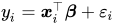
線形回帰モデル 、を考えてみましょう。つまり、、ここで、は行が観測値に対応し、列が独立変数または説明変数に対応する設計行列です。独立観測値のてこ比スコアは次のように与えられます。 ${\displaystyle {y}_{i}={\boldsymbol {x}}_{i}^{\top }{\boldsymbol {\beta }}+{\varepsilon }_{i}}$${\displaystyle i=1,\,2,\ldots ,\,n}$${\displaystyle {\boldsymbol {y}}=\mathbf {X} {\boldsymbol {\beta }}+{\boldsymbol {\varepsilon }}}$${\displaystyle \mathbf {X} }$${\displaystyle n\times p}$ ${\displaystyle {i}^{th}}$${\displaystyle {\boldsymbol {x}}_{i}}$

${\displaystyle h_{ii}=\left[\mathbf {H} \right]_{ii}={\boldsymbol {x}}_{i}^{\top }\left(\mathbf {X} ^{\top }\mathbf {X} \right)^{-1}{\boldsymbol {x}}_{i}}$、正射影行列（別名ハット行列）の対角要素。${\displaystyle {i}^{th}}$${\displaystyle \mathbf {H} =\mathbf {X} \left(\mathbf {X} ^{\top }\mathbf {X} \right)^{-1}\mathbf {X} ^{\top }}$

したがって、レバレッジスコアは、 の平均に対する の 間の「加重」距離として見ることができます （マハラノビス距離との関係を参照）。また、測定された（従属）値（つまり、 ）が適合された（予測された）値（つまり、 ）に影響を与える度合いとして解釈することもできます。数学的には、 ${\displaystyle {i}^{th}}$${\displaystyle {\boldsymbol {x}}_{i}}$${\displaystyle {\boldsymbol {x}}_{i}}$${\displaystyle {i}^{th}}$${\displaystyle y_{i}}$${\displaystyle {i}^{th}}$${\displaystyle {\widehat {y\,}}_{i}}$

${\displaystyle h_{ii}={\frac {\partial {\widehat {y\,}}_{i}}{\partial y_{i}}}}$。

したがって、レバレッジスコアは、観測自己感度または自己影響とも呼ばれます。^[3]上記の式で(つまり、予測はの範囲空間へのの正射影である)という事実を使用すると、 が得られます。このレバレッジは、すべての観測の説明変数の値に依存しますが、従属変数の値には依存しないことに注意してください。 ${\displaystyle {\boldsymbol {\widehat {y}}}={\mathbf {H} }{\boldsymbol {y}}}$${\displaystyle {\boldsymbol {\widehat {y}}}}$${\displaystyle {\boldsymbol {y}}}$${\displaystyle \mathbf {X} }$${\displaystyle h_{ii}=\left[\mathbf {H} \right]_{ii}}$${\displaystyle (\mathbf {X} )}$${\displaystyle (y_{i})}$

1. レバレッジは  0 から 1 の間の数値です。証明:はべき等行列( ) かつ対称行列 ( )であることに注意してください。したがって、 という事実を使用することで、 が得られます。 であることがわかっているので、 が得られます。${\displaystyle h_{ii}}$${\displaystyle 0\leq h_{ii}\leq 1.}$
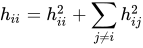
   ${\displaystyle \mathbf {H} }$${\displaystyle \mathbf {H} ^{2}=\mathbf {H} }$${\displaystyle h_{ij}=h_{ji}}$${\displaystyle \left[\mathbf {H} ^{2}\right]_{ii}=\left[\mathbf {H} \right]_{ii}}$${\displaystyle h_{ii}=h_{ii}^{2}+\sum _{j\neq i}h_{ij}^{2}}$${\displaystyle \sum _{j\neq i}h_{ij}^{2}\geq 0}$${\displaystyle h_{ii}\geq h_{ii}^{2}\implies 0\leq h_{ii}\leq 1}$
2. レバレッジの合計は、（切片を含む）のパラメータの数に等しくなります。証明:。${\displaystyle (p)}$${\displaystyle {\boldsymbol {\beta }}}$
   ${\displaystyle \sum _{i=1}^{n}h_{ii}=\operatorname {Tr} (\mathbf {H} )=\operatorname {Tr} \left(\mathbf {X} \left(\mathbf {X} ^{\top }\mathbf {X} \right)^{-1}\mathbf {X} ^{\top }\right)=\operatorname {Tr} \left(\mathbf {X} ^{\top }\mathbf {X} \left(\mathbf {X} ^{\top }\mathbf {X} \right)^{-1}\right)=\operatorname {Tr} (\mathbf {I} _{p})=p}$

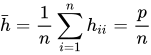
大きなレバレッジは、極端なに対応します。一般的なルールは、レバレッジ値が平均レバレッジの 2 倍以上であるを特定することです(上記の特性 2 を参照)。つまり、 の場合、は外れ値と見なされます。統計学者の中 には、 ではなく のしきい値を好む人もいます。 ${\displaystyle {h_{ii}}}$${\displaystyle {{\boldsymbol {x}}_{i}}}$${\displaystyle {{\boldsymbol {x}}_{i}}}$${\displaystyle {h}_{ii}}$${\displaystyle {\bar {h}}={\dfrac {1}{n}}\sum _{i=1}^{n}h_{ii}={\dfrac {p}{n}}}$${\displaystyle h_{ii}>2{\dfrac {p}{n}}}$${\displaystyle {{\boldsymbol {x}}_{i}}}$${\displaystyle 3p/{n}}$${\displaystyle 2p/{n}}$

レバレッジはマハラノビス距離と密接な関係があります（証明^[4]）。具体的には、ある行列に対して、長さ の平均のベクトルからの（ の行） の マハラノビス距離の2乗は で、 は の推定 共分散行列です。これは、1の列ベクトルを追加した後のハット行列のレバレッジと関係があります。2つの関係は次のとおりです。 ${\displaystyle n\times p}$${\displaystyle \mathbf {X} }$${\displaystyle {{\boldsymbol {x}}_{i}}}$${\displaystyle {\boldsymbol {x}}_{i}^{\top }}$${\displaystyle {i}^{th}}$${\displaystyle \mathbf {X} }$${\displaystyle {\widehat {\boldsymbol {\mu }}}=\sum _{i=1}^{n}{\boldsymbol {x}}_{i}}$${\displaystyle p}$${\displaystyle D^{2}({\boldsymbol {x}}_{i})=({\boldsymbol {x}}_{i}-{\widehat {\boldsymbol {\mu }}})^{\top }\mathbf {S} ^{-1}({\boldsymbol {x}}_{i}-{\widehat {\boldsymbol {\mu }}})}$${\displaystyle \mathbf {S} =\mathbf {X} ^{\top }\mathbf {X} }$${\displaystyle {{\boldsymbol {x}}_{i}}}$${\displaystyle h_{ii}}$${\displaystyle \mathbf {X} }$

${\displaystyle D^{2}({\boldsymbol {x}}_{i})=(n-1)(h_{ii}-{\tfrac {1}{n}})}$

この関係により、レバレッジを意味のある要素に分解することができ、高いレバレッジの原因を分析的に調査できるようになります。^[5]

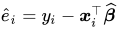
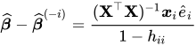
回帰分析では、てこ関数と影響関数を組み合わせて、1つのデータポイントを削除した場合に推定係数がどの程度変化するかを計算します。回帰残差を と表すと、式^{[6] [7]}を使用して推定係数を1つ除外した推定係数と比較することができます。${\displaystyle {\widehat {e}}_{i}=y_{i}-{\boldsymbol {x}}_{i}^{\top }{\widehat {\boldsymbol {\beta }}}}$${\displaystyle {\widehat {\boldsymbol {\beta }}}}$${\displaystyle {\widehat {\boldsymbol {\beta }}}^{(-i)}}$

${\displaystyle {\widehat {\boldsymbol {\beta }}}-{\widehat {\boldsymbol {\beta }}}^{(-i)}={\frac {(\mathbf {X} ^{\top }\mathbf {X} )^{-1}{\boldsymbol {x}}_{i}{\widehat {e}}_{i}}{1-h_{ii}}}}$

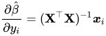
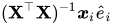
Young (2019) は、残差制御後のこの式のバージョンを使用しています。^[8]この式を直感的に理解するには、が観測値が回帰パラメータに影響を及ぼす可能性を捉えていること、したがって、回帰パラメータに対するその観測値の適合値からの偏差の実際の影響を捉えていることに注目してください。次に、式は で割って、観測値を調整するのではなく削除するという事実を考慮に入れています。これは、除去によって共変量の分布がより変化するという事実を反映しており、レバレッジの高い観測値（つまり、外れ値の共変量値）に適用した場合、共変量の分布がより変化するという事実を反映しています。回帰コンテキストで統計的影響関数の一般的な式を適用すると、同様の式が生まれます。^{[9] [10]}${\displaystyle {\frac {\partial {\hat {\beta }}}{\partial y_{i}}}=(\mathbf {X} ^{\top }\mathbf {X} )^{-1}{\boldsymbol {x}}_{i}}$${\displaystyle (\mathbf {X} ^{\top }\mathbf {X} )^{-1}{\boldsymbol {x}}_{i}{\widehat {e}}_{i}}$${\displaystyle (1-h_{ii})}$

固定された等 分散回帰誤差を持つ通常の最小二乗設定の場合、回帰残差は分散を持つ。 ${\displaystyle \mathbf {X} }$ ${\displaystyle \varepsilon _{i},}$ ${\displaystyle {\boldsymbol {y}}=\mathbf {X} {\boldsymbol {\beta }}+{\boldsymbol {\varepsilon }};\ \ \operatorname {Var} ({\boldsymbol {\varepsilon }})=\sigma ^{2}\mathbf {I} }$${\displaystyle {i}^{th}}$ ${\displaystyle e_{i}=y_{i}-{\widehat {y}}_{i}}$

${\displaystyle \operatorname {Var} (e_{i})=(1-h_{ii})\sigma ^{2}}$。

言い換えれば、観測値のてこ比スコアは、その観測値に対するモデルの予測誤りのノイズの度合いを決定し、てこ比が高いほどノイズは少なくなります。これは、がべき等かつ対称であり、したがって であるという事実から導かれます。 ${\displaystyle \mathbf {I} -\mathbf {H} }$${\displaystyle {\widehat {\boldsymbol {y}}}=\mathbf {H} {\boldsymbol {y}}}$${\displaystyle \operatorname {Var} ({\boldsymbol {e}})=\operatorname {Var} ((\mathbf {I} -\mathbf {H} ){\boldsymbol {y}})=(\mathbf {I} -\mathbf {H} )\operatorname {Var} ({\boldsymbol {y}})(\mathbf {I} -\mathbf {H} )^{\top }=\sigma ^{2}(\mathbf {I} -\mathbf {H} )^{2}=\sigma ^{2}(\mathbf {I} -\mathbf {H} )}$

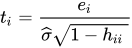
対応するスチューデント化残差（観測値固有の推定残差分散を調整した残差）は、

${\displaystyle t_{i}={e_{i} \over {\widehat {\sigma }}{\sqrt {1-h_{ii}\ }}}}$

ここで はの適切な推定値です。 ${\displaystyle {\widehat {\sigma }}}$${\displaystyle \sigma }$

部分レバレッジ( PL ) は、各観測値の総レバレッジに対する個々の独立変数の寄与度を測る尺度です。つまり、PL は、変数としての変更が回帰モデルにどの程度追加されるかの尺度です。次のように計算されます。 ${\displaystyle h_{ii}}$

${\displaystyle \left(\mathrm {PL} _{j}\right)_{i}={\frac {\left(\mathbf {X} _{j\bullet [j]}\right)_{i}^{2}}{\sum _{k=1}^{n}\left(\mathbf {X} _{j\bullet [j]}\right)_{k}^{2}}}}$

ここで、は独立変数のインデックス、は観測のインデックス、は残りの独立変数に対する回帰からの残差です。部分的てこ比は、変数の部分回帰プロット内の点のてこ比であることに注意してください。独立変数の部分的てこ比が大きいデータ ポイントは、自動回帰モデル構築手順でその変数の選択に過度の影響を及ぼす可能性があります。 ${\displaystyle j}$${\displaystyle i}$${\displaystyle \mathbf {X} _{j\bullet [j]}}$${\displaystyle \mathbf {X} _{j}}$${\displaystyle {i}^{th}}$${\displaystyle {j}^{th}}$

R、Pythonなどの多くのプログラムや統計パッケージには、Leverage の実​​装が含まれています。

• 投影行列- その主な対角要素は観測値のてこである
• マハラノビス距離–測地基準系の影響力の(スケール化された) 尺度
• 部分的レバレッジ
• クックの距離– 観測値が削除されたときの回帰係数の変化の尺度
• DFFITS
• 外れ値– 極端なY値を持つ観測値
• 自由度（統計）、レバレッジスコアの合計