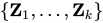
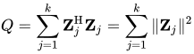
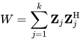
定義
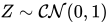
複素標準正規乱数 標準複素正規乱数 または標準複素ガウス乱数 は複素乱数である。Z {\displaystyle Z} 1 / 2 {\displaystyle 1/2} 3 ] : [ 4 ] : に
どこ⊥ ⊥ {\displaystyle \perp \!\!\!\perp } Z ~ C N ( 0 、 1 ) {\displaystyle Z\sim {\mathcal {CN}}(0,1)} Z {\displaystyle Z}
複素正規乱数 仮定するX {\displaystyle X} Y {\displaystyle Y} ( X 、 Y ) T {\displaystyle (X,Y)^{\mathrm {T} }} 正規乱数ベクトル である。すると複素乱数変数はZ = X + 私 Y {\displaystyle Z=X+iY} これは複素正規確率変数 または複素ガウス確率変数 と呼ばれる。[ 3 ] :
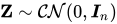
複素標準正規乱数ベクトル n次元複素ランダムベクトルZ = ( Z 1 、 … 、 Z n ) T {\displaystyle \mathbf {Z} =(Z_{1},\ldots ,Z_{n})^{\mathrm {T} }} 複素標準正規乱数ベクトル または複素標準ガウス乱数ベクトル である。 [ 3 ] : [ 4 ] : Z {\displaystyle \mathbf {Z} } Z ~ C N ( 0 、 私 n ) {\displaystyle \mathbf {Z} \sim {\mathcal {CN}}(0,{\boldsymbol {I}}_{n})}
複素正規乱数ベクトル もしX = ( X 1 、 … 、 X n ) T \displaystyle \mathbf {X} =(X_{1},\ldots ,X_{n})^{\mathrm {T} }} Y = ( Y 1 、 … 、 Y n ) T {\displaystyle \mathbf {Y} =(Y_{1},\ldots ,Y_{n})^{\mathrm {T} }} ランダムベクトル ですR n \displaystyle \mathbb {R} ^{n}} [ X 、 Y ] {\displaystyle [\mathbf {X} ,\mathbf {Y} ]} 、 2 n {\displaystyle 2n} コンポーネント。次に、複素ランダムベクトル は
Z = X + 私 Y {\displaystyle \mathbf {Z} =\mathbf {X} +i\mathbf {Y} \,} は複素正規ランダムベクトル または複素ガウスランダムベクトル です。
密度関数 複素正規分布の確率密度関数は次のように計算できます。
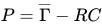
f ( z ) = 1 π n 検出 ( Γ ) 検出 ( P ) exp { − 1 2 [ z − μ z ¯ − μ ¯ ] H [ Γ C C ¯ Γ ¯ ] − 1 [ z − μ z ¯ − μ ¯ ] } = 検出 ( P − 1 ¯ − R * P − 1 R ) 検出 ( P − 1 ) π n e − ( z − μ ) * P − 1 ¯ ( z − μ ) + 再 ( ( z − μ ) ⊺ R ⊺ P − 1 ¯ ( z − μ ) ) 、 {\displaystyle {\begin{aligned}f(z)&={\frac {1}{\pi ^{n}{\sqrt {\det(\Gamma )\det(P)}}}}\,\exp \!\left\{-{\frac {1}{2}}{\begin{bmatrix}z-\mu \\{\overline {z}}-{\overline {\mu }}\end{bmatrix}}^{\mathrm {H} }{\begin{bmatrix}\Gamma &C\\{\overline {C}}&{\overline {\Gamma }}\end{bmatrix}}^{\!\!-1}\!{\begin{bmatrix}z-\mu \\{\overline {z}}-{\overline {\mu }}\end{bmatrix}}\right\}\\[8pt]&={\tfrac {\sqrt {\det \left({\overline {P^{-1}}}-R^{\ast }P^{-1}R\right)\det(P^{-1})}}{\pi ^{n}}}\,e^{-(z-\mu )^{\ast }{\overline {P^{-1}}}(z-\mu )+\operatorname {Re} \left((z-\mu )^{\intercal }R^{\intercal }{\overline {P^{-1}}}(z-\mu )\right)},\end{aligned}}} どこR = C H Γ − 1 {\displaystyle R=C^{\mathrm {H} }\Gamma ^{-1}} P = Γ ¯ − R C {\displaystyle P={\overline {\Gamma }}-RC}
特性関数 複素正規分布の特性関数は [ 5 ]で与えられる。
φ ( w ) = exp { 私 再 ( w ¯ ′ μ ) − 1 4 ( w ¯ ′ Γ w + 再 ( w ¯ ′ C w ¯ ) ) } 、 {\displaystyle \varphi (w)=\exp \!{\big \{}i\operatorname {Re} ({\overline {w}}'\mu )-{\tfrac {1}{4}}{\big (}{\overline {w}}'\Gamma w+\operatorname {Re} ({\overline {w}}'C{\overline {w}}){\big )}{\big \}},} 議論がw {\displaystyle w} これはn 次元の複素ベクトルです。
物件 もしZ {\displaystyle \mathbf {Z} } n 次元ベクトルであり、A {\displaystyle {\boldsymbol {A}}} ×n 行列、b {\displaystyle b} m ベクトル、次に線形変換A Z + b {\displaystyle {\boldsymbol {A}}\mathbf {Z} +b} Z ~ C N ( μ 、 Γ 、 C ) ⇒ A Z + b ~ C N ( A μ + b 、 A Γ A H 、 A C A T ) {\displaystyle Z\ \sim \ {\mathcal {CN}}(\mu ,\,\Gamma ,\,C)\quad \Rightarrow \quad AZ+b\ \sim \ {\mathcal {CN}}(A\mu +b,\,A\Gamma A^{\mathrm {H} },\,ACA^{\mathrm {T} })} もしZ {\displaystyle \mathbf {Z} } n ベクトルである。 2 [ ( Z − μ ) H P − 1 ¯ ( Z − μ ) − 再 ( ( Z − μ ) T R T P − 1 ¯ ( Z − μ ) ) ] ~ χ 2 ( 2 n ) {\displaystyle 2{\Big [}(\mathbf {Z} -\mu )^{\mathrm {H} }{\overline {P^{-1}}}(\mathbf {Z} -\mu )-\operatorname {Re} {\big (}(\mathbf {Z} -\mu )^{\mathrm {T} }R^{\mathrm {T} }{\overline {P^{-1}}}(\mathbf {Z} -\mu ){\big )}{\Big ]}\ \sim \ \chi ^{2}(2n)} 中心極限定理 。Z 1 、 … 、 Z T {\displaystyle Z_{1},\ldots ,Z_{T}} T ( 1 T ∑ t = 1 T Z t − E [ Z t ] ) → d C N ( 0 、 Γ 、 C ) 、 {\displaystyle {\sqrt {T}}{\Big (}{\tfrac {1}{T}}\textstyle \sum _{t=1}^{T}Z_{t}-\operatorname {E} [Z_{t}]{\Big )}\ {\xrightarrow {d}}\ {\mathcal {CN}}(0,\,\Gamma ,\,C),} どこΓ = E [ Z Z H ] {\displaystyle \Gamma =\operatorname {E} [ZZ^{\mathrm {H} }]} C = E [ Z Z T ] {\displaystyle C=\operatorname {E} [ZZ^{\mathrm {T} }]}
円対称の中央ケース
実部と虚部の分配 もしZ = X + 私 Y {\displaystyle \mathbf {Z} =\mathbf {X} +i\mathbf {Y} } [ X 、 Y ] {\displaystyle [\mathbf {X} ,\mathbf {Y} ]}
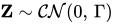
( X Y ) ~ N ( [ 0 0 ] 、 1 2 [ 再 Γ − 私は Γ 私は Γ 再 Γ ] ) {\displaystyle {\begin{pmatrix}\mathbf {X} \\\mathbf {Y} \end{pmatrix}}\ \sim \ {\mathcal {N}}{\Big (}{\begin{bmatrix}0\\0\end{bmatrix}},\ {\tfrac {1}{2}}{\begin{bmatrix}\operatorname {Re} \,\Gamma &-\operatorname {Im} \,\Gamma \\\operatorname {Im} \,\Gamma &\operatorname {Re} \,\Gamma \end{bmatrix}}{\Big )}} どこΓ = E [ Z Z H ] {\displaystyle \Gamma =\operatorname {E} [\mathbf {Z} \mathbf {Z} ^{\mathrm {H} }]}
参考文献 ↑ Goodman, NR (1963). "Statistical analysis based on a certain multivariate complex Gaussian distribution (an introduction)" . The Annals of Mathematical Statistics . 34 (1): 152– 177. doi : 10.1214/aoms/1177704250 . JSTOR 2991290 . ↑ 書籍の章、Gallager.R 、9ページ。1 2 3 4 5 6 Lapidoth, A. (2009). デジタルコミュニケーションの基礎 . Cambridge University Press. ISBN 9780521193955 。1 2 3 4 Tse, David (2005). ワイヤレス通信の基礎 . Cambridge University Press. ISBN 9781139444668 。1 2 3 Picinbono, Bernard (1996). "2次複素ランダムベクトルと正規分布" . IEEE Transactions on Signal Processing . 44 (10): 2637– 2640. Bibcode : 1996ITSP...44.2637P . doi : 10.1109/78.539051 . ↑ Daniel Wollschlaeger. "The Hoyt Distribution (Documentation for R package 'shotGroups' version 0.6.2)" . ↑ 書籍の章、Gallager.R










![{\displaystyle [\mathbf {X} ,\mathbf {Y} ]}](https://wikimedia.org/api/rest_v1/media/math/render/svg/39633a1d2cf0edd432b5ceee258360ac47ebf9db)


![{\displaystyle \mu =\operatorname {E} [\mathbf {Z} ],\quad \Gamma =\operatorname {E} [(\mathbf {Z} -\mu )({\mathbf {Z} }-\mu )^{\mathrm {H} }],\quad C=\operatorname {E} [(\mathbf {Z} -\mu )(\mathbf {Z} -\mu )^{\mathrm {T} }],}](https://wikimedia.org/api/rest_v1/media/math/render/svg/d8186b266f6fa5b1c962c01bcc77a666d4ae579b)






![{\displaystyle {\begin{aligned}&V_{XX}\equiv \operatorname {E} [(\mathbf {X} -\mu _{X})(\mathbf {X} -\mu _{X})^{\mathrm {T} }]={\tfrac {1}{2}}\operatorname {Re} [\Gamma +C],\quad V_{XY}\equiv \operatorname {E} [(\mathbf {X} -\mu _{X})(\mathbf {Y} -\mu _{Y})^{\mathrm {T} }]={\tfrac {1}{2}}\operatorname {Im} [-\Gamma +C],\\&V_{YX}\equiv \operatorname {E} [(\mathbf {Y} -\mu _{Y})(\mathbf {X} -\mu _{X})^{\mathrm {T} }]={\tfrac {1}{2}}\operatorname {Im} [\Gamma +C],\quad \,V_{YY}\equiv \operatorname {E} [(\mathbf {Y} -\mu _{Y})(\mathbf {Y} -\mu _{Y})^{\mathrm {T} }]={\tfrac {1}{2}}\operatorname {Re} [\Gamma -C],\end{aligned}}}](https://wikimedia.org/api/rest_v1/media/math/render/svg/7816194d319a6f156db69f13e9f2add16b9937fe)

![{\displaystyle {\begin{aligned}f(z)&={\frac {1}{\pi ^{n}{\sqrt {\det(\Gamma )\det(P)}}}}\,\exp \!\left\{-{\frac {1}{2}}{\begin{bmatrix}z-\mu \\{\overline {z}}-{\overline {\mu }}\end{bmatrix}}^{\mathrm {H} }{\begin{bmatrix}\Gamma &C\\{\overline {C}}&{\overline {\Gamma }}\end{bmatrix}}^{\!\!-1}\!{\begin{bmatrix}z-\mu \\{\overline {z}}-{\overline {\mu }}\end{bmatrix}}\right\}\\[8pt]&={\tfrac {\sqrt {\det \left({\overline {P^{-1}}}-R^{\ast }P^{-1}R\right)\det(P^{-1})}}{\pi ^{n}}}\,e^{-(z-\mu )^{\ast }{\overline {P^{-1}}}(z-\mu )+\operatorname {Re} \left((z-\mu )^{\intercal }R^{\intercal }{\overline {P^{-1}}}(z-\mu )\right)},\end{aligned}}}](https://wikimedia.org/api/rest_v1/media/math/render/svg/736e45cbaf3e68d9ca78dbb9cafda0402ed3c4b3)





![{\displaystyle 2{\Big [}(\mathbf {Z} -\mu )^{\mathrm {H} }{\overline {P^{-1}}}(\mathbf {Z} -\mu )-\operatorname {Re} {\big (}(\mathbf {Z} -\mu )^{\mathrm {T} }R^{\mathrm {T} }{\overline {P^{-1}}}(\mathbf {Z} -\mu ){\big )}{\Big ]}\ \sim \ \chi ^{2}(2n)}](https://wikimedia.org/api/rest_v1/media/math/render/svg/a4752c39ed434c1a5f987accdda45de63384153f)

![\displaystyle {\sqrt {T}}{\Big (}{\tfrac {1}{T}}\textstyle \sum _{t=1}^{T}Z_{t}-\operatorname {E} [Z_{t}]{\Big )}\ \xrightarrow {d} \ {\mathcal {CN}}(0,\,\Gamma ,\,C),}](https://wikimedia.org/api/rest_v1/media/math/render/svg/7a8e03845ead334b995c22f8fb6a63887477b36d)
![{\displaystyle \Gamma =\演算子名 {E} [ZZ^{\mathrm {H} }]}](https://wikimedia.org/api/rest_v1/media/math/render/svg/040fb5df40ce465da42594603d54e851879ccdf9)
![{\displaystyle C=\operatorname {E} [ZZ^{\mathrm {T} }]}](https://wikimedia.org/api/rest_v1/media/math/render/svg/d57ca27eba4a64bb77bac89459414af49a542522)




![{\displaystyle \Gamma =\演算子名 {E} [\mathbf {Z} \mathbf {Z} ^{\mathrm {H} }]}](https://wikimedia.org/api/rest_v1/media/math/render/svg/5664837bef03da1b45373e4aefa316892ccf80ed)






![{\displaystyle [-\pi ,\pi ]}](https://wikimedia.org/api/rest_v1/media/math/render/svg/cb064fd6c55820cfa660eabeeda0f6e3c4935ae6)