Okun's law

In economics, Okun's law is an empirically observed relationship between unemployment and losses in a country's production. It is named after Arthur Melvin Okun, who first proposed the relationship in 1962.^[1] The "gap version" states that for every 1% increase in the unemployment rate, a country's GDP will experience a roughly 2% decrease on its potential GDP. The "difference version"^[2] describes the relationship between quarterly changes in unemployment and quarterly changes in real GDP. The stability and usefulness of the law has been disputed.^[3]

Okun's law is an empirical relationship. In Okun's original statement of his law, a 2% increase in output corresponds to a 1% decline in the rate of cyclical unemployment; a 0.5% increase in labor force participation; a 0.5% increase in hours worked per employee; and a 1% increase in output per hours worked (labor productivity).^[4]

Okun's law states that a one-point increase in the cyclical unemployment rate is associated with two percentage points of negative growth in real GDP. The relationship varies depending on the country and time period under consideration.

The relationship has been tested by regressing GDP or GNP growth on change in the unemployment rate. Martin Prachowny estimated about a 3% decrease in output for every 1% increase in the unemployment rate.^[5] However, he argued that the majority of this change in output is actually due to changes in factors other than unemployment, such as capacity utilization and hours worked. Holding these other factors constant reduces the association between unemployment and GDP to around 0.7% for every 1% change in the unemployment rate. The magnitude of the decrease seems to be declining over time in the United States. According to Andrew Abel and Ben Bernanke, estimates based on data from more recent years give about a 2% decrease in output for every 1% increase in unemployment.^[6]

GDPの増減が失業率の増減よりも速い場合がある理由はいくつかあります。

失業率が上昇するにつれて、

• 従業員からの資金循環によって生じる乗数効果の低下
• 失業者は労働力から脱落する（求職活動をやめる）ことがあり、その場合、失業統計には含まれなくなる。
• 雇用されている労働者は労働時間が短くなる可能性がある
• 労働生産性は低下する可能性がある。おそらく雇用主が必要以上に多くの労働者を抱え込むためだろう。

オークンの法則が示唆するところの一つは、労働生産性の向上や労働力人口の増加は、実質的な純生産量が純失業率の低下を伴わずに増加する可能性があるということである（「雇用なき成長」現象）。

オオクンの法則は、ルーカスウェッジと混同されることがある。

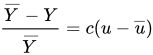
オオクンの法則のギャップ版は、次のように記述できる（Abel & Bernanke 2005）。

${\displaystyle {\frac {{\overline {Y}}-Y}{\overline {Y}}}=c(u-{\overline {u}})}$、 どこ

• ${\displaystyle Y}$実際の出力
• ${\displaystyle {\overline {Y}}}$潜在GDP
• ${\displaystyle u}$実際の失業率は
• ${\displaystyle {\overline {u}}}$自然失業率
• ${\displaystyle c}$失業率の変化と生産量の変化を関連付ける要因は

1955年頃から米国では、cの値は概ね2か3程度であったと、前述のとおりである。

上記のように、オオクンの法則のギャップバージョンは、実際には使いにくい。${\displaystyle {\overline {Y}}}$そして${\displaystyle {\overline {u}}}$ 推定することはできても、測定することはできません。オオクンの法則のより一般的な形式である、差分法則または成長率法則として知られるものは、生産量の変化と失業率の変化の関係を示しています。

${\displaystyle {\frac {\Delta Y}{Y}}=kc\,\Delta u\,}$、 どこ：

• ${\displaystyle Y}$そして${\displaystyle c}$上記で定義されているとおりである。
• ${\displaystyle \Delta Y}$実際の生産量が前年から翌年にかけて変化した値です。
• ${\displaystyle \Delta u}$実際の失業率が前年から翌年にかけてどのように変化するかを示す指標である。
• ${\displaystyle k}$は完全雇用生産量の年間平均成長率である。

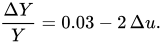
現在、米国ではkは約3%、cは約2なので、方程式は次のように書ける。

${\displaystyle {\frac {\Delta Y}{Y}}=0.03-2\,\Delta u.\,}$

この記事冒頭のグラフは、オークンの法則の成長率を示したもので、年単位ではなく四半期単位で測定されています。

まず、オオクンの法則の最初の形式から始めましょう。

${\displaystyle {\frac {{\overline {Y}}-Y}{\overline {Y}}}=1-{\frac {Y}{\overline {Y}}}=c(u-{\overline {u}})}$

${\displaystyle {\frac {Y}{\overline {Y}}}-1=c({\overline {u}}-u).}$

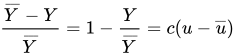
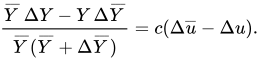
両辺の年間差を取ると、

${\displaystyle \Delta \left({\frac {Y}{\overline {Y}}}\right)={\frac {Y+\Delta Y}{{\overline {Y}}+\Delta {\overline {Y}}}}-{\frac {Y}{\overline {Y}}}=c(\Delta {\overline {u}}-\Delta u).}$

両方の分子を共通分母で割ると、次の式が得られます。

${\displaystyle {\frac {{\overline {Y}}\,\Delta Y-Y\,\Delta {\overline {Y}}}{{\overline {Y}}({\overline {Y}}+\Delta {\overline {Y}})}}=c(\Delta {\overline {u}}-\Delta u).}$

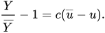
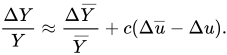
左辺に${\displaystyle {\frac {{\overline {Y}}+\Delta {\overline {Y}}}{Y}}}$はほぼ1に等しいので、

${\displaystyle {\frac {{\overline {Y}}\Delta Y-Y\Delta {\overline {Y}}}{{\overline {Y}}Y}}={\frac {\Delta Y}{Y}}-{\frac {\Delta {\overline {Y}}}{\overline {Y}}}\approx c(\Delta {\overline {u}}-\Delta u)}$

${\displaystyle {\frac {\Delta Y}{Y}}\approx {\frac {\Delta {\overline {Y}}}{\overline {Y}}}+c(\Delta {\overline {u}}-\Delta u).}$

私たちは次のように仮定します${\displaystyle \Delta {\overline {u}}}$自然失業率の変化は、ほぼ0に等しいと仮定します。また、${\displaystyle {\frac {\Delta {\overline {Y}}}{\overline {Y}}}}$完全雇用生産高の成長率は、その平均値とほぼ等しい。${\displaystyle k}$最終的に私たちは

${\displaystyle {\frac {\Delta Y}{Y}}\approx k-c\,\Delta u.}$

実際のデータと理論的な予測を比較すると、オークンの法則は失業率と実質GDPの傾向を予測する上で非常に貴重なツールであることが証明されています。しかし、オークンの法則によって理論的に証明されたデータの精度は、現実世界の数値と比較すると、一般的に不正確であることが証明されています。これは、オークンの係数のばらつきによるものです。オーストラリア準備銀行を含む多くの人々は、オークンの法則によって証明された情報は、ある程度許容できると結論付けています。^{[ 7 ]}また、オークンの法則は、長期予測よりも短期予測の方が精度が高い傾向があるという結論に至った研究結果もあります。予測担当者は、オークンの係数に影響を与える可能性のある予期せぬ市場状況のために、これが真実であると結論付けています。

そのため、オークンの法則は、長期的な分析や正確な数値計算に用いるというよりは、失業率と実質GDPの間の短期的な傾向分析のためのツールとして、予測担当者に一般的に受け入れられている。

サンフランシスコ連邦準備銀行は、1970年代、1990年代、2000年代の過去の景気後退の経験的データを用いて、オークンの法則が有用な理論であると判断した。すべての景気後退は、リアルタイムデータと修正データの両方で反時計回りのループという2つの共通の主要な傾向を示した。1990年代と2000年代の回復では、ループはより小さく、よりタイトであった。^{[ 8 ]}

• ルーカスウェッジ

• Ball, Laurence ; Tovar Jalles, João; Loungani, Prakash. 「予測者はオークンの法則を信じているか？失業率と生産量予測の評価」(PDF) . imf.org . 国際通貨基金. 2016年7月11日取得.
• アベル、アンドリュー・B. & バーナンキ、ベン・S. (2005).マクロ経済学（第5版）. ピアソン・アディソン・ウェスリー. ISBN 0-321-16212-9。
• ベイリー、マーティン・ニール＆オクン、アヴナー・A. (1965) 『失業とインフレとの闘い：現代経済の問題』 ニューヨーク：WWノートン社；ISBN 0-393-95055-7（1983年；第3版改訂版）
• Case, Karl E. & Fair, Ray C. (1999).経済学原理（第5版）. Prentice-Hall. ISBN 0-13-961905-4。
• オクン、アヴナー A. (1962). 「潜在的GNP、その測定と意義」 . カウルズ財団、イェール大学。
• プロッサー、チャールズ・I.、シュワート、G・ウィリアム（1979）。「潜在GNP：その測定と意義：異論」、カーネギー・ロチェスター公共政策会議シリーズ
• Knotek, Edward S. 「オークンの法則はどれほど有用か」『エコノミック・レビュー』カンザスシティ連邦準備銀行、2007年第4四半期、73-103頁 。
• Prachowny, Martin FJ (1993). 「オークンの法則：理論的基礎と改訂推定」、 『経済統計レビュー』、75 (2)、pp. 331 –336。
• ゴードン、ロバート・J.、『生産性、成長、インフレ、失業』、ケンブリッジ大学出版局、2004年
• マクブライド、ビル（2010年10月11日）「実質GDP成長率と失業率」 Calculated Risk。2010年12月5日取得。
• 後藤英治ブルギ、コンスタンティン。「セクターオークンの法則と各国の景気循環の違い」(PDF) 。2020-09-09に取得。
• Ball, Laurence; Leigh, Daniel; Loungani, Prakash. 「オークンの法則：50歳で健康？（PDF） 」。 2020年9月9日取得。