カルボ（段階的）契約

カルボ契約とは、マクロ経済学において、企業が名目価格を設定する際に、価格が最後にリセットされてからの時間に関係なく、企業が価格をリセットできる一定の確率が存在するという価格設定モデルに与えられた名称である。このモデルは、ギレルモ・カルボが1983年の論文「効用最大化フレームワークにおける段階的価格設定」で初めて提唱した。^{[ 1 ]}元の論文は連続時間数学フレームワーク で書かれていたが、現在では主に離散時間バージョンが使用されている。カルボモデルは、ニューケインズ派DSGEマクロ経済モデルにおける名目価格の硬直性をモデル化する最も一般的な方法である。

企業が任意の期間に価格を再設定できる確率をh (ハザード率) と定義するか、あるいは同等に、その期間に価格が変更されない確率 ( 1-h ) (生存率) と定義することができます。この文脈では、確率hは「カルボ確率」と呼ばれることもあります。カルボモデルの重要な特徴は、価格設定者が名目価格がどのくらいの期間維持されるかを知らないことです。現在の価格がちょうど i 期間続く確率は、

${\displaystyle \mathrm {Pr} [i]=(1-h)^{i-1}h}$

したがって、i 回の連続した期間を生き残る確率は幾何分布に従い、名目価格が最初に設定されてからの期待期間は次のようになる。 ${\displaystyle E[\mathrm {Pr} [i]]=h^{-1}}$例えば、カルボ確率hが1期間あたり0.25の場合、期待される持続期間は4期間です。カルボ確率は一定であり、価格が設定されてからの経過時間に依存しないため、i期間以上存続する確率は、すべての期間においてまったく同じ幾何分布によって与えられます。${\displaystyle i=1,\dotsc ,\infty }$したがって、h = 0.25 の場合、価格がどれだけ古いかに関わらず、さらに 4 期間続くことが期待されます。

カルボモデルでは、ショックに対する価格の反応は時間とともに広がります。ショックが時間tで経済を襲ったとします。価格のhの割合はすぐに反応し、残りの(1-h)は固定されたままです。次の期間には、まだ ${\displaystyle (1-h)^{2}}$ショックに反応せず、その場に留まった人々。ショック後の期間、縮小した人々は${\displaystyle (1-h)^{i}}$一定期間が経過した後でも、価格が変化せず固定されたままの一定割合の企業が存在します。これは、契約期間が固定されているテイラーモデル（例えば4期間）とは対照的です。テイラーモデルでは、4期間後には企業は価格を再設定します。

カルボ価格モデルは、1995年にジョン・ロバーツによってニューケインジアン・フィリップス曲線が導出された際に重要な役割を果たし、 ^{[ 2 ]}それ以来、ニューケインジアンDSGEモデルで使用されています。^{[ 3 ] [ 4 ]}

${\displaystyle \pi _{t}=\beta E_{t}[\pi _{t+1}]+\kappa y_{t}\qquad {\mbox{ニューケインジアン・フィリップス曲線}}}$

どこ

${\displaystyle \kappa ={\frac {h[1-(1-h)\beta ]}{1-h}}\gamma }$。

次期インフレ率の現在の予想は、${\displaystyle \beta E_{t}[\pi _{t+1}]}$係数${\displaystyle \kappa }$これは、現在のインフレ率が現在の生産量にどれだけ反応するかを捉えたものです。ニューケインジアン・フィリップス曲線は、価格決定が将来を見据えたものであり、現在のインフレ率に影響を与えるのは、現在の需要水準（生産量で表される）だけでなく、将来の予想インフレ率も含まれるという事実を反映しています。

経済における名目価格の硬直性を測定する方法はいくつかある。企業（価格設定者）は多数存在し、価格を頻繁に変更する企業もあれば、そうでない企業もある。たとえ「通常」価格をめったに変更しない企業であっても、通常価格に戻る前に短期間の特別価格やセールを実施することがある。

公称剛性を測定する方法として提案されている2つの方法^{[ 5 ]}は以下のとおりです。

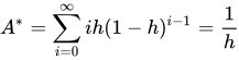
(i)契約の平均経過期間。すべての企業を対象に、価格が現在の水準に設定されている期間を尋ねることができます。カルボ価格設定では、すべての企業が同じハザード率hを持つと仮定すると、h の割合がちょうどリセットされたばかりであり、h.(1-h)の割合が前の期間にリセットされ、今期も固定されたままであり、一般に、i 期間前に設定された価格のうち今日まで存続している割合は次のように与えられます。 $\displaystyle \alpha ^{i}}$、 どこ：

${\displaystyle \alpha ^{i}=(1-h)^{i-1}h}$

契約の平均経過年数${\displaystyle A^{*}}$すると

${\displaystyle A^{*}=\sum _{i=0}^{\infty }ih(1-h)^{i-1}={\frac {1}{h}}}$

契約の平均経過期間は、名目上の硬直性を測る指標の一つです。しかし、この指標には中断バイアスという問題があります。つまり、ある時点において、価格が現在の水準に留まっている期間しか観測できないのです。そこで、次の価格変動時に契約の完了期間がどれくらいになるかを知りたいと思うかもしれません。これが2つ目の指標です。

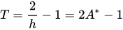
(ii) The average completed length of contracts. This is similar to the average age in that it looks at the current prices set by firms. However, rather than asking how long was it since the price was last set (the age of the contract), it asks how long will the price have lasted when the price next changes. Clearly for a single firm, this is random. Across all firms, however, the Law of large numbers kicks in and we can calculate the exact distribution of completed contract lengths. It can be shown that^[6] the average completed length of contracts is given by T:

${\displaystyle T={\frac {2}{h}}-1=2A^{*}-1}$

That is, the completed length of contracts is twice the average age minus 1. Thus, for example, if h= 0.25, 25% of prices change each period. At any time, the average age of prices will be 4 periods. However, the corresponding average completed length of contracts is 7 periods.

One of the major problems with the Calvo contract as a model of pricing is that the inflation dynamics it results in do not fit the data. Inflation is better described by the hybrid new Keyensian Phillips curve which includes lagged inflation:

${\displaystyle \pi _{t}=(1-\psi )\beta E_{t}[\pi _{t+1}]+\psi \pi _{t-1}+\kappa y_{t}\qquad {\mbox{ハイブリッド・ニューケインジアン・フィリップス曲線}}}$

This has led to the original Calvo model to be developed in a number of directions:

(a) Indexation. With indexation, prices are automatically updated in response to lagged inflation (at least to some degree), which gives rise to the hybrid new Keyensian Phillips curve. The Calvo probability refers to the firm being able to choose the price it sets that period (which happens with probability ${\displaystyle h}$) or to have the price rise by indexation (which happens with probability ${\displaystyle (1-h)}$. The Calvo model with indexation is adopted by many new Keynesian researchers.^[7][8][9]

(b) Duration dependent hazard function${\displaystyle h(i)}$. A key feature of the Calvo model is that the hazard rate is constant: the probability of changing the price does not depend on how old the price is. In 1999, Wolman suggested that the model should be generalized to allow for the hazard rate to vary with the duration.^[10] The key idea is that an older price may be more or less likely to change than a newer price, which is captured by the hazard function h(i) which allows the hazard rate to be a function of age i. This generalized Calvo model with duration dependent hazard rate has been developed by several authors.^[11][12]

• Taylor contract (economics)

• デイビッド・ローマー著『上級マクロ経済学』マグロウヒル・ハイヤー・エデュケーション刊、第4版（2011年5月1日）ISBN 978-0073511375。
• カール・ウォルシュ著『金融理論と政策』（第3版）、MIT Press、2010年、ISBN 978-0262013772。
• マイケル・ウッドフォード著『貨幣利子と物価』プリンストン大学出版局、2003年、ISBN 9781400830169。