カントロヴィッチの定理

カントロヴィッチの定理、またはニュートン・カントロヴィッチの定理は、ニュートン法の半局所収束に関する数学的な定理である。この定理は、1948年にレオニード・カントロヴィッチによって初めて提唱された。^{[1] [2]この定理は、}バナッハの不動点定理の形式に似ているが、不動点ではなく零点の存在と一意性を述べている。^[3]

ニュートン法は、ある条件下で方程式の解または方程式系のベクトル解に収束する点の列を構築する。カントロビッチの定理は、この列の初期点に関する条件を与える。これらの条件が満たされると、初期点の近くに解が存在し、列はその点に収束する。^{[1] [2]}${\displaystyle x}$${\displaystyle f(x)=0}$${\displaystyle F(x)=0}$

を開集合とし、ヤコビアンが局所的にリプシッツ連続である微分可能関数とする（例えば、が2回微分可能である場合）。つまり、任意のに対して開集合が存在し、任意のに対してとなる定数が存在すると仮定する。${\displaystyle X\subset \mathbb {R} ^{n}}$${\displaystyle F:X\subset \mathbb {R} ^{n}\to \mathbb {R} ^{n}}$ ${\displaystyle F^{\prime }(\mathbf {x} )}$${\displaystyle F}$${\displaystyle x\in X}$${\displaystyle U\subset X}$${\displaystyle x\in U}$${\displaystyle L>0}$${\displaystyle \mathbf {x} ,\mathbf {y} \in U}$

${\displaystyle \|F'(\mathbf {x} )-F'(\mathbf {y} )\|\leq L\;\|\mathbf {x} -\mathbf {y} \|}$

が成り立つ。左辺のノルムは演算子ノルムである。言い換えれば、任意のベクトルに対して不等式 ${\displaystyle \mathbf {v} \in \mathbb {R} ^{n}}$

${\displaystyle \|F'(\mathbf {x} )(\mathbf {v} )-F'(\mathbf {y} )(\mathbf {v} )\|\leq L\;\|\mathbf { x} -\mathbf {y} \|\,\|\mathbf {v} \|}$

保持する必要があります。

ここで任意の初期点を選択する。 が可逆であると仮定し、ニュートンステップを構築する。${\displaystyle \mathbf {x} _{0}\in X}$${\displaystyle F'(\mathbf {x} _{0})}$${\displaystyle \mathbf {h} _{0}=-F'(\mathbf {x} _{0})^{-1}F(\mathbf {x} _{0}).}$

次の仮定は、次の点だけでなく、球全体が集合 内に含まれているということです。をこの球上のヤコビアンのリプシッツ定数とします (存在すると仮定)。 ${\displaystyle \mathbf {x} _{1}=\mathbf {x} _{0}+\mathbf {h} _{0}}$${\displaystyle B(\mathbf {x} _{1},\|\mathbf {h} _{0}\|)}$${\displaystyle X}$${\displaystyle M}$

最後の準備として、可能な限り、シーケンス、、を次のよう に再帰的に構築します。${\displaystyle (\mathbf {x} _{k})_{k}}$${\displaystyle (\mathbf {h} _{k})_{k}}$${\displaystyle (\alpha _{k})_{k}}$

${\displaystyle {\begin{alignedat}{2}\mathbf {h} _{k}&=-F'(\mathbf {x} _{k})^{-1}F(\mathbf {x} _ {k})\\[0.4em]\alpha _{k}&=M\,\|F'(\mathbf {x} _{k})^{-1}\|\,\|\mathbf {h} _{k}\|\\[0.4em]\mathbf {x} _{k+1}&=\mathbf {x } _{k}+\mathbf {h} _{k}.\end{alignedat}}}$

さて、もしそうなら ${\displaystyle \alpha _{0}\leq {\tfrac {1}{2}}}$

1. の解は閉じた球体の中に存在し、${\displaystyle \mathbf {x} ^{*}}$${\displaystyle F(\mathbf {x} ^{*})=0}$${\displaystyle {\bar {B}}(\mathbf {x} _{1},\|\mathbf {h} _{0}\|)}$
2. から始まるニュートン反復法は、少なくとも線形収束の順序でに収束します。${\displaystyle \mathbf {x} _{0}}$${\displaystyle \mathbf {x} ^{*}}$

より正確だが証明が少し難しいステートメントは、二次多項式の 根を使用する。${\displaystyle t^{\ast }\leq t^{**}}$

${\displaystyle p(t)=\left({\tfrac {1}{2}}L\|F'(\mathbf {x} _{0})^{-1}\|^{-1}\right)t^{2}-t+\|\mathbf {h} _{0}\|}$、

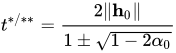
${\displaystyle t^{\ast /**}={\frac {2\|\mathbf {h} _{0}\|}{1\pm {\sqrt {1-2\alpha _{0}}}}}}$

およびその比率

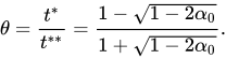
${\displaystyle \theta ={\frac {t^{*}}{t^{**}}}={\frac {1-{\sqrt {1-2\alpha _{0}}}}{1+{\sqrt {1-2\alpha _{0}}}}}.}$

それから

1. 閉じた球の中に解が存在する${\displaystyle \mathbf {x} ^{*}}$${\displaystyle {\bar {B}}(\mathbf {x} _{1},\theta \|\mathbf {h} _{0}\|)\subset {\bar {B}}(\mathbf {x} _{0},t^{*})}$
2. 大きなボールの中にあるユニークなもの${\displaystyle B(\mathbf {x} _{0},t^{*\ast })}$
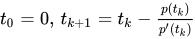
3. の解への収束は、2次多項式のニュートン反復がその最小根に収束することによって支配される。^[4]ならば、 ${\displaystyle F}$${\displaystyle p(t)}$${\displaystyle t^{\ast }}$${\displaystyle t_{0}=0,\,t_{k+1}=t_{k}-{\tfrac {p(t_{k})}{p'(t_{k})}}}$

   ${\displaystyle \|\mathbf {x} _{k+p}-\mathbf {x} _{k}\|\leq t_{k+p}-t_{k}.}$

4. 二次収束は誤差推定から得られる^[5]

   ${\displaystyle \|\mathbf {x} _{n+1}-\mathbf {x} ^{*}\|\leq \theta ^{2^{n}}\|\mathbf {x} _{n+1}-\mathbf {x} _{n}\|\leq {\frac {\theta ^{2^{n}}}{2^{n}}}\|\mathbf {h} _{0}\|.}$

1986年に山本は、ドーリング（1969）、オストロフスキー（1971、1973）、^{[6] [7]}グラッグ・タピア（1974）、ポトラ・プタク（1980）、^[8]ミエル（1981）、^[9]ポトラ（1984）、^[10]などのニュートン法の誤差評価がカントロビッチの定理から導かれることを証明した。^[11]

カントロヴィッチの定理にはq類似物がある。 ^{[12] [13]}その他の一般化/変形については、Ortega & Rheinboldt (1970)を参照。^[14]

大石と田辺は、カントロヴィッチの定理は線形計画法の信頼できる解を得るために適用できると主張した。^[15]

• John H. HubbardおよびBarbara Burke Hubbard : Vector Calculus, Linear Algebra, and Differential Forms: A Unified Approach、Matrix Editions、ISBN 978-0-9715766-3-6 (第 3 版のプレビューと Kant.-thm. を含むサンプル資料) 
• 山本哲郎 (2001) 「ニュートン法およびニュートン類似法の収束解析の歴史的発展」 Brezinski, C.、Wuytack, L. (編) 『数値解析: 20 世紀の歴史的発展』 North- Holland、pp. 241–263。ISBN 0-444-50617-9。