アイデア
深層推論 シーケント計算 では、各推論規則は論理式の最上位レベルの論理結合子のみを生成/削除できます。つまり、ほとんどの部分式は変更されません。一方、深層推論では、各推論規則は任意のレベルの部分式を書き換えることができます。
例えば、古典論理のシーケント計算では、規則Γ 、 A 、 B ⊢ Δ Γ 、 A ∧ B ⊢ Δ {\displaystyle {\frac {\Gamma ,A,B\vdash \Delta }{\Gamma ,A\land B\vdash \Delta }}} A 、 B {\displaystyle A,B} 結合子のみが A ∧ B {\displaystyle A\land B}
深層推論の場合、推論ルールは構文ツリー内の任意の深さの任意のサブ式に適用できます。言い換えれば、構文ツリー 内のすべてのノードのうち、A ∧ B {\displaystyle A\land B}
上から下への対称性 シーケント計算と自然演繹 において、証明は推論規則の木構造である。これにより、根本的な非対称性が生じる。証明木の最上位は多数の葉シーケントから構成されるが、最下位は単一の末端シーケントである。しかしながら、多くの推論規則は対称的である。上半分と下半分は相互に導出可能である。
例えば、ルールを適用できる場合Γ ⊢ A Γ ⊢ B Γ ⊢ A & B ( ⊢ & ) {\displaystyle {\frac {\Gamma \vdash A\quad \Gamma \vdash B}{\Gamma \vdash A\&B}}(\vdash \&)} Γ ⊢ A & B {\displaystyle \Gamma \vdash A\&B} Γ ⊢ A {\displaystyle \Gamma \vdash A} Γ ⊢ B {\displaystyle \Gamma \vdash B} ⊢ & {\displaystyle \vdash \&}
シーケント計算の形式は、シーケントの並置によってこのトップダウン対称性を暗黙のうちに示している。Γ ⊢ A {\displaystyle \Gamma \vdash A} Γ ⊢ B {\displaystyle \Gamma \vdash B} 証明計算の対象レベル には存在しないことを意味する。
シーケントの計算においては、証明とは推論規則の列である。これにより、トップダウンの対称性がオブジェクトレベルに配置される。
SKSg
意味 SKSgは古典命題論理のためのCoSである。
SKSgのシンボルは以下の通り:
原子1 0 、 1 ¯ 0 、 1 1 、 1 ¯ 1 、 … {\displaystyle a_{0},{\bar {a}}_{0},a_{1},{\bar {a}}_{1},\dots } 1 私 、 1 ¯ 私 {\displaystyle a_{i},{\bar {a}}_{i}} 接続詞∨ 、 ∧ {\displaystyle \lor ,\land } ユニット⊤ 、 ⊥ {\displaystyle \top ,\bot } SKSgでは否定は存在しません。なぜなら、否定を論理結合子から単なる論理原子間のペアリングへと格下げしたからです。
SKSgの構造は、バッカス・ナウア記法 において以下の構文を持つ。F ::= 1 | 1 ¯ | ⊤ | ⊥ | F ∨ F | F ∧ F {\displaystyle F::=a|{\bar {a}}|\top |\bot |F\lor F|F\land F}
構造の双対性は次のように定義される。1 ¯ = 1 ¯ 、 1 ¯ ¯ = 1 A ∧ B ¯ = A ¯ ∨ B ¯ 、 A ∨ B ¯ = A ¯ ∧ B ¯ {\displaystyle {\begin{aligned}{\overline {a}}={\bar {a}},&\quad {\overline {\bar {a}}}=a\\{\overline {A\land B}}={\overline {A}}\lor {\overline {B}},&\quad {\overline {A\lor B}}={\overline {A}}\land {\overline {B}}\end{aligned}}} 、 3つの双対ペアで構成されています。
2つの論理 推論規則は自己双対関係にある。
これらの規則に加えて、以下の式があります。A ∨ B = B ∨ A A ∧ B = B ∧ A ( A ∨ B ) ∨ C = A ∨ ( B ∨ C ) ( A ∧ B ) ∧ C = A ∧ ( B ∧ C ) A ∨ ⊥ = A A ∧ ⊤ = A ⊤ ∨ ⊤ = ⊤ ⊥ ∧ ⊥ = ⊥ {\displaystyle {\begin{array}{rcl}A\lor B&=&B\lor A\\A\land B&=&B\land A\\(A\lor B)\lor C&=&A\lor (B\lor C)\\(A\land B)\land C&=&A\land (B\land C)\end{array}}\qquad {\begin{array}{rcl}A\lor \bot &=&A\\A\land \top &=&A\\\top \lor \top &=&\top \\\bot \land \bot &=&\bot \end{array}}\quad }
不動産 これは有効な導出です。 ( 1 ∨ b ) ∧ 1 ‖ ( ( 1 ∨ b ) ∧ 1 ) ∧ ( ( 1 ∨ b ) ∧ 1 ) ≡ ( ( 1 1 ∧ 1 ( c ↑ ) ) ∨ ( b b ∧ b ( c ↑ ) ) ( 1 ∨ b ) ∧ ( 1 ∨ b ) ( m ) ) ∧ ( 1 1 ∧ 1 ( c ↑ ) ) 。 {\displaystyle {\begin{array}{c}(a\lor b)\land a\\\Vert \\((a\lor b)\land a)\land ((a\lor b)\land a)\end{array}}\equiv \left({\frac {\left({\frac {a}{a\land a}}\;(\mathrm {c} \uparrow )\right)\lor \left({\frac {b}{b\land b}}\;(\mathrm {c} \uparrow )\right)}{(a\lor b)\land (a\lor b)}}\;(\mathrm {m} )\right)\land \left({\frac {a}{a\land a}}\;(\mathrm {c} \uparrow )\right)\quad .} 構造ルール
カットフリー 導出とは、次の導出である。私 ↑ {\displaystyle \mathrm {i} \uparrow } 分割 と呼ばれる技術によってカットをなくす ことができます。[ 3 ] [ 4 ]
MLL⁻ を単位のない 乗法線形論理 の証明システムと定義する。
式は以下から構成されるF ::= 1 | 1 ¯ | F ⅋ F | F × F {\displaystyle F::=a|{\bar {a}}|F\mathbin {\mbox{⅋}} F|F\times F} 1 {\displaystyle a} 1 ¯ {\displaystyle {\bar {a}}} ( A ⊗ B ) ⊥ = A ⊥ ⅋ B ⊥ 、 ( A ⅋ B ) ⊥ = A ⊥ ⊗ B ⊥ {\displaystyle (A\otimes B)^{\bot }=A^{\bot }\mathbin {\mbox{⅋}} B^{\bot },\quad (A\mathbin {\mbox{⅋}} B)^{\bot }=A^{\bot }\otimes B^{\bot }} 1 ¯ ¯ = 1 {\displaystyle {\bar {\bar {a}}}=a}
このシステムのCoSは以下のとおりです。[ 4 ] 私 ↓ A ⊥ ⅋ A 私 ↑ A ⊗ A ⊥ 私 ↓ S { B } S { ( A ⊥ ⅋ A ) ⊗ B } 私 ↑ S { B ⅋ ( A ⊗ A ⊥ ) } S { B } σ ↓ S { A ⅋ B } S { B ⅋ A } σ ↑ S { A ⊗ B } S { B ⊗ A } α ↓ S { A ⅋ ( B ⅋ C ) } S { ( A ⅋ B ) ⅋ C } α ↑ S { A ⊗ ( B ⊗ C ) } S { ( A ⊗ B ) ⊗ C } s S { A ⊗ ( B ⅋ C ) } S { ( A ⊗ B ) ⅋ C } {\displaystyle {\begin{aligned}&\mathrm {i} \downarrow \;{\frac {}{A^{\perp }\mathbin {\mbox{⅋}} A}}&&\mathrm {i} \uparrow \;{\frac {A\otimes A^{\perp }}{}}\\&\mathrm {i} \downarrow \;{\frac {S\{B\}}{S\{(A^{\perp }\mathbin {\mbox{⅋}} A)\otimes B\}}}&&\mathrm {i} \uparrow \;{\frac {S\{B\mathbin {\mbox{⅋}} (A\otimes A^{\perp })\}}{S\{B\}}}\\&\sigma \downarrow \;{\frac {S\{A\mathbin {\mbox{⅋}} B\}}{S\{B\mathbin {\mbox{⅋}} A\}}}&&\sigma \uparrow \;{\frac {S\{A\otimes B\}}{S\{B\otimes A\}}}\\&\alpha \downarrow \;{\frac {S\{A\mathbin {\mbox{⅋}} (B\mathbin {\mbox{⅋}} C)\}}{S\{(A\mathbin {\mbox{⅋}} B)\mathbin {\mbox{⅋}} C\}}}&&\alpha \uparrow \;{\frac {S\{A\otimes (B\otimes C)\}}{S\{(A\otimes B)\otimes C\}}}\\&\mathrm {s} \;{\frac {S\{A\otimes (B\mathbin {\mbox{⅋}} C)\}}{S\{(A\otimes B)\mathbin {\mbox{⅋}} C\}}}\end{aligned}}}
開始ルールは4つあり、i↑用が2つ、i↓用が2つです。ルールが1つではなく2つある理由は、このシステムには単位がないためです。1 、 ⊥ {\displaystyle 1,\bot } 1 {\displaystyle 1} ⊗ {\displaystyle \otimes } A ⊥ ⅋ A {\displaystyle {\frac {}{A^{\perp }\mathbin {\mbox{⅋}} A}}} S { B } S { ( A ⊥ ⅋ A ) ⊗ B } {\displaystyle {\frac {S\{B\}}{S\{(A^{\perp }\mathbin {\mbox{⅋}} A)\otimes B\}}}} S { − } {\displaystyle S\{-\}} B = 1 {\displaystyle B=1} ⊥ {\displaystyle \bot } ⅋ {\displaystyle \mathbin {\mbox{⅋}} } A ⊗ A ⊥ {\displaystyle {\frac {A\otimes A^{\bot }}{}}} S { B ⅋ ( A ⊗ A ⊥ ) } S { B } {\displaystyle {\frac {S\{B\mathbin {\mbox{⅋}} (A\otimes A^{\perp })\}}{S\{B\}}}}
協会の規則α {\displaystyle \alpha } σ {\displaystyle \sigma } ( A ⊗ B ) ⊗ C = A ⊗ ( B ⊗ C ) {\displaystyle (A\otimes B)\otimes C=A\otimes (B\otimes C)}
i↑はシーケント計算における恒等公理に対応する。A ⊢ A {\displaystyle A\vdash A} ⊢ A ⊥ 、 A {\displaystyle \vdash A^{\bot },A}
i↓ はカットルールに対応します。Γ ⊢ Δ 、 A A 、 Γ ′ ⊢ Δ ′ Γ 、 Γ ′ ⊢ Δ 、 Δ ′ {\displaystyle {\frac {\Gamma \vdash \Delta ,A\quad A,\Gamma '\vdash \Delta '}{\Gamma ,\Gamma '\vdash \Delta ,\Delta '}}}
スイッチルールS { A ⊗ ( B ⅋ C ) } S { ( A ⊗ B ) ⅋ C } {\displaystyle {\frac {S\{A\otimes (B\mathbin {\mbox{⅋}} C)\}}{S\{(A\otimes B)\mathbin {\mbox{⅋}} C\}}}} S { A ⊗ ( B ⅋ C ) } ⊢ S { ( A ⊗ B ) ⅋ C } {\displaystyle S\{A\otimes (B\mathbin {\mbox{⅋}} C)\}\vdash S\{(A\otimes B)\mathbin {\mbox{⅋}} C\}}
解釈 MLL⁻では、記号は⊗ 、 ⅋ {\displaystyle \otimes ,\mathbin {\mbox{⅋}} } ⅋ {\displaystyle \mathbin {\mbox{⅋}} } ⊢ Γ 、 A 、 B 、 Δ ⊢ Γ 、 A ⅋ B 、 Δ {\displaystyle {\frac {\vdash \Gamma ,A,B,\Delta }{\vdash \Gamma ,A\mathbin {\mbox{⅋}} B,\Delta }}} ⊗ {\displaystyle \otimes } ⊢ Γ 、 A ⊢ B 、 Δ ⊢ Γ 、 A ⊗ B 、 Δ {\displaystyle {\frac {\vdash \Gamma ,A\quad \vdash B,\Delta }{\vdash \Gamma ,A\otimes B,\Delta }}}
MLL⁻ の CoS では、シンボル⊗ {\displaystyle \otimes } ⊗ {\displaystyle \otimes } ⅋ {\displaystyle \mathbin {\mbox{⅋}} }
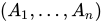
特に、MLL⁻シーケント計算の証明木が与えられた場合、各シーケントを変換すれば、それをMLL⁻CoSの証明に変換することができる。⊢ A 1 、 … 、 A n {\displaystyle \vdash A_{1},\dots ,A_{n}} A 1 ⅋ … ⅋ A n {\displaystyle A_{1}\mathbin {\mbox{⅋}} \dots \mathbin {\mbox{⅋}} A_{n}} ⊢ Γ 1 … ⊢ Γ n {\displaystyle \vdash \Gamma _{1}\quad \dots \quad \vdash \Gamma _{n}} Γ 1 ⊗ ⋯ ⊗ Γ n {\displaystyle \Gamma _{1}\otimes \dots \otimes \Gamma _{n}}
カット除去はi↓除去に対応する。
SLLS SLLSシステムは、完全な線形論理 のCoSバージョンです。MLL⁻のCoSよりもはるかに大きいです。[ 5 ] 1 私 ↓ 1 1 ⅋ 1 ¯ 1 私 ↑ 1 ⊗ 1 ¯ ⊥ d ↓ ( A ⅋ B ) & ( C ⅋ D ) ( A & C ) ⅋ ( B ⊕ D ) d ↑ ( A ⊕ B ) ⊗ ( C & D ) ( A ⊗ C ) ⊕ ( B ⊗ D ) p ↓ ! ( R ⅋ T ) ! R ⅋ ? T p ↑ ! R ⊗ ? T ? ( R ⊗ T ) 1 w ↓ 0 1 1 c ↓ 1 ⊕ 1 1 1 c ↑ 1 1 & 1 1 w ↑ 1 ⊤ n m ↓ 0 0 & 0 s ( A ⅋ B ) ⊗ C ( A ⊗ C ) ⅋ B m ( A & B ) ⊕ ( C & D ) ( A ⊕ C ) & ( B ⊕ D ) n m ↑ ⊤ ⊕ ⊤ ⊤ n m 1 ↓ 0 0 ⅋ 0 m 1 ↓ ( A ⅋ B ) ⊕ ( C ⅋ D ) ( A ⊕ C ) ⅋ ( B ⊕ D ) m 1 ↑ ( A & B ) ⊗ ( C & D ) ( A ⊗ C ) & ( B ⊗ D ) n m 1 ↑ ⊤ ⊗ ⊤ ⊤ n m 2 ↓ 0 0 ⊗ 0 m 2 ↓ ( A ⊗ B ) ⊕ ( C ⊗ D ) ( A ⊕ C ) ⊗ ( B ⊕ D ) m 2 ↑ ( A & B ) ⅋ ( C & D ) ( A ⅋ C ) & ( B ⅋ D ) n m 2 ↑ ⊤ ⅋ ⊤ ⊤ n l 1 ↓ 0 ? 0 l 1 ↓ ? R ⊕ ? T ? ( R ⊕ T ) l 1 ↑ ! ( R & T ) ! R & ! T n l 1 ↑ ! ⊤ ⊤ n l 2 ↓ 0 ! 0 l 2 ↓ ! R ⊕ ! T ! ( R ⊕ T ) l 2 ↑ ? ( R & T ) ? R & ? T n l 2 ↑ ? ⊤ ⊤ n z ↓ ⊥ ? 0 z ↓ ? R ⅋ T ? ( R ⊕ T ) z ↑ ! ( R & T ) ! R ⊗ T n z ↑ ! ⊤ 1 {\displaystyle {\begin{aligned}&\mathrm {ai} \downarrow \;{\frac {1}{a\mathbin {\mbox{⅋}} {\bar {a}}}}&&\mathrm {ai} \uparrow \;{\frac {a\otimes {\bar {a}}}{\bot }}\\&\mathrm {d} \downarrow \;{\frac {(A\mathbin {\mbox{⅋}} B)\mathbin {\&} (C\mathbin {\mbox{⅋}} D)}{(A\mathbin {\&} C)\mathbin {\mbox{⅋}} (B\oplus D)}}&&\mathrm {d} \uparrow \;{\frac {(A\oplus B)\otimes (C\mathbin {\&} D)}{(A\otimes C)\oplus (B\otimes D)}}\\&\mathrm {p} \downarrow \;{\frac {!(R\mathbin {\mbox{⅋}} T)}{!R\mathbin {\mbox{⅋}} ?T}}&&\mathrm {p} \uparrow \;{\frac {!R\otimes ?T}{?(R\otimes T)}}\\&\mathrm {aw} \downarrow \;{\frac {0}{a}}&&\mathrm {ac} \downarrow \;{\frac {a\oplus a}{a}}&&\mathrm {ac} \uparrow \;{\frac {a}{a\mathbin {\&} a}}&&\mathrm {aw} \uparrow \;{\frac {a}{\top }}\\&\mathrm {nm} \downarrow \;{\frac {0}{0\mathbin {\&} 0}}&&\mathrm {s} \;{\frac {(A\mathbin {\mbox{⅋}} B)\otimes C}{(A\otimes C)\mathbin {\mbox{⅋}} B}}&&\mathrm {m} \;{\frac {(A\mathbin {\&} B)\oplus (C\mathbin {\&} D)}{(A\oplus C)\mathbin {\&} (B\oplus D)}}&&\mathrm {nm} \uparrow \;{\frac {\top \oplus \top }{\top }}\\&\mathrm {nm} _{1}\downarrow \;{\frac {0}{0\mathbin {\mbox{⅋}} 0}}&&\mathrm {m} _{1}\downarrow \;{\frac {(A\mathbin {\mbox{⅋}} B)\oplus (C\mathbin {\mbox{⅋}} D)}{(A\oplus C)\mathbin {\mbox{⅋}} (B\oplus D)}}&&\mathrm {m} _{1}\uparrow \;{\frac {(A\mathbin {\&} B)\otimes (C\mathbin {\&} D)}{(A\otimes C)\mathbin {\&} (B\otimes D)}}&&\mathrm {nm} _{1}\uparrow \;{\frac {\top \otimes \top }{\top }}\\&\mathrm {nm} _{2}\downarrow \;{\frac {0}{0\otimes 0}}&&\mathrm {m} _{2}\downarrow \;{\frac {(A\otimes B)\oplus (C\otimes D)}{(A\oplus C)\otimes (B\oplus D)}}&&\mathrm {m} _{2}\uparrow \;{\frac {(A\mathbin {\&} B)\mathbin {\mbox{⅋}} (C\mathbin {\&} D)}{(A\mathbin {\mbox{⅋}} C)\mathbin {\&} (B\mathbin {\mbox{⅋}} D)}}&&\mathrm {nm} _{2}\uparrow \;{\frac {\top \mathbin {\mbox{⅋}} \top }{\top }}\\&\mathrm {nl} _{1}\downarrow \;{\frac {0}{?0}}&&\mathrm {l} _{1}\downarrow \;{\frac {?R\oplus ?T}{?(R\oplus T)}}&&\mathrm {l} _{1}\uparrow \;{\frac {!(R\mathbin {\&} T)}{!R\mathbin {\&} !T}}&&\mathrm {nl} _{1}\uparrow \;{\frac {!\top }{\top }}\\&\mathrm {nl} _{2}\downarrow \;{\frac {0}{!0}}&&\mathrm {l} _{2}\downarrow \;{\frac {!R\oplus !T}{!(R\oplus T)}}&&\mathrm {l} _{2}\uparrow \;{\frac {?(R\mathbin {\&} T)}{?R\mathbin {\&} ?T}}&&\mathrm {nl} _{2}\uparrow \;{\frac {?\top }{\top }}\\&\mathrm {nz} \downarrow \;{\frac {\bot }{?0}}&&\mathrm {z} \downarrow \;{\frac {?R\mathbin {\mbox{⅋}} T}{?(R\oplus T)}}&&\mathrm {z} \uparrow \;{\frac {!(R\mathbin {\&} T)}{!R\otimes T}}&&\mathrm {nz} \uparrow \;{\frac {!\top }{1}}\end{aligned}}}
A ⊗ B = B ⊗ A ( A ⊗ B ) ⊗ C = A ⊗ ( B ⊗ C ) A ⊗ 1 = A A & B = B & A ( A & B ) & C = A & ( B & C ) A & ⊤ = A A ⊕ B = B ⊕ A ( A ⊕ B ) ⊕ C = A ⊕ ( B ⊕ C ) A ⊕ 0 = A A ⅋ B = B ⅋ A ( A ⅋ B ) ⅋ C = A ⅋ ( B ⅋ C ) A ⅋ 1 = ⊥ ? ? R = ? R ! ! R = ! R ⊥ ⊕ ⊥ = ⊥ = ? ⊥ 1 & 1 = 1 = ! 1 {\displaystyle {\begin{aligned}A\otimes B&=B\otimes A&\qquad (A\otimes B)\otimes C&=A\otimes (B\otimes C)&\qquad A\otimes 1&=A\\A\mathbin {\&} B&=B\mathbin {\&} A&(A\mathbin {\&} B)\mathbin {\&} C&=A\mathbin {\&} (B\mathbin {\&} C)&A\mathbin {\&} \top &=A\\A\oplus B&=B\oplus A&(A\oplus B)\oplus C&=A\oplus (B\oplus C)&A\oplus 0&=A\\A\mathbin {\mbox{⅋}} B&=B\mathbin {\mbox{⅋}} A&(A\mathbin {\mbox{⅋}} B)\mathbin {\mbox{⅋}} C&=A\mathbin {\mbox{⅋}} (B\mathbin {\mbox{⅋}} C)&A\mathbin {\mbox{⅋}} 1&=\bot \\??R&=?R&!!R&=!R\\\bot \oplus \bot &=\bot =?\bot &1\mathbin {\&} 1&=1=!1\end{aligned}}}
BV このCoSによりBVシステム(基本システムV)を生成できます:[ 1 ] 1 私 ↓ ∘ 1 ⅋ 1 ¯ 1 私 ↑ 1 ⊗ 1 ¯ ∘ s ( A ⅋ B ) ⊗ C ( A ⊗ C ) ⅋ B q ↓ ( A ⅋ B ) ◃ ( C ⅋ D ) ( A ◃ C ) ⅋ ( B ◃ D ) q ↑ ( A ◃ B ) ⊗ ( C ◃ D ) ( A ⊗ C ) ◃ ( B ⊗ D ) {\displaystyle {\begin{aligned}&\mathrm {ai} \downarrow \;{\frac {\circ }{a\mathbin {\mbox{⅋}} {\bar {a}}}}&&\mathrm {ai} \uparrow \;{\frac {a\otimes {\bar {a}}}{\circ }}\\&\mathrm {s} \;{\frac {(A\mathbin {\mbox{⅋}} B)\otimes C}{(A\otimes C)\mathbin {\mbox{⅋}} B}}\\&\mathrm {q} \downarrow \;{\frac {(A\mathbin {\mbox{⅋}} B)\triangleleft (C\mathbin {\mbox{⅋}} D)}{(A\triangleleft C)\mathbin {\mbox{⅋}} (B\triangleleft D)}}&&\mathrm {q} \uparrow \;{\frac {(A\triangleleft B)\otimes (C\triangleleft D)}{(A\otimes C)\triangleleft (B\otimes D)}}\end{aligned}}}
A ⊗ B = B ⊗ A ( A ⊗ B ) ⊗ C = A ⊗ ( B ⊗ C ) A ⊗ ∘ = A A ⅋ B = B ⅋ A ( A ⅋ B ) ⅋ C = A ⅋ ( B ⅋ C ) A ⅋ ∘ = A ( A ◃ B ) ◃ C = A ◃ ( B ◃ C ) A ◃ ∘ = A = ∘ ◃ A {\displaystyle {\begin{aligned}A\otimes B&=B\otimes A&\qquad (A\otimes B)\otimes C&=A\otimes (B\otimes C)&\qquad A\otimes \circ &=A\\A\mathbin {\mbox{⅋}} B&=B\mathbin {\mbox{⅋}} A&(A\mathbin {\mbox{⅋}} B)\mathbin {\mbox{⅋}} C&=A\mathbin {\mbox{⅋}} (B\mathbin {\mbox{⅋}} C)&A\mathbin {\mbox{⅋}} \circ &=A\\&&(A\triangleleft B)\triangleleft C&=A\triangleleft (B\triangleleft C)&A\triangleleft \circ &=A=\circ \triangleleft A\end{aligned}}}
参考文献 1 2 Guglielmi, Alessio (2007-01-01). "相互作用と構造のシステム" . ACM Trans. Comput. Logic . 8 (1): 1–es. arXiv : cs/9910023 . doi : 10.1145/1182613.1182614 . ISSN 1529-3785 . ↑ Novaković, Novak; Straßburger, Lutz (2015-04-21). "On the Power of Substitution in the Calculus of Structures" . ACM Trans. Comput. Logic . 16 (3): 19:1–19:20. doi : 10.1145/2701424 . ISSN 1529-3785 . ↑ 「ディープ推論」 。alessio.guglielmi.name 。 2026年4月30 日 取得 。 1 2 Strassburger, Lutz (2006-11-20). "証明ネットと証明の同一性". arXiv : cs/0610123 . ↑ Aler Tubella, Andrea; Straßburger, Lutz (2019). 深層推論入門:ESSLLI'19 講義ノート、2019 年 8 月 5 日~16 日、ラトビア大学 (PDF) (レポート)。
さらに読む カイ・ブリュンラー(2004)。古典的証明における深層推論と対称性 。ロゴス出版。 


![{\displaystyle []}](https://wikimedia.org/api/rest_v1/media/math/render/svg/0261e8d17bc0832139076efdad67e7c0abf21cff)

![{\displaystyle [A_{1},\dots ,A_{n}]}](https://wikimedia.org/api/rest_v1/media/math/render/svg/291ed428307f4caeaf674ce67e20cca5de5fdcc7)





